Updated by Chainika Thakar (Originally written by Mandeep Kaur)
Since predicting the future stock prices in the stock market is crucial for the investors, Time Series and its related concepts hold an exceptional quality of organizing the data for accurate prediction. In this article, let us read through the importance of Time Series, its analysis and forecasting.
Here, some of the essential subtopics covered are:
- What is Time Series and Time Series Analysis?
- Types of Time Series
- What are the Components of Time Series Analysis?
- Structures for the Components or Decomposing
- What is Time Series Forecasting?
- How to Import, Calculate & Plot and Validate Time Series in Python for Forecasting?
- Time Series Analysis: Working with Date-Time Data in Python
- Mean Reversion in Time Series Analysis
What is Time Series and Time Series Analysis
In simple words, Time Series is a sequence of observations over time, which are usually spaced at regular intervals. To support the statement, here are some of the examples of Time Series:
- Daily stock prices for the last 5 years
- 1-minute stock price data for the last 90 days
- Quarterly revenues of a company over the last 10 years
- Monthly car sales of an automaker for the last 3 years
- The annual unemployment rate of a state in the last 50 years
Coming to Time Series analysis, it simply implies identifying those methods which help in the analysis of Time Series data.
The main aim of the Time Series Analysis is to develop those models that best capture or describe the Time Series or data set. Also, this leads to an understanding of the underlying causes of the dataset to help you create meaningful and accurate forecasts. You can also learn to obtain, visualise, and analyse stock market data.
Also, there are few types of Time Series which we will see ahead.
Types of Time Series
Let us now look at the types of Time Series that a dataset can belong to:
- Univariate & Multivariate
- Stationary & Non-Stationary
Univariate & Multivariate
A Univariate Time Series refers to the set of observations over time of a single variable. One important thing to note here is that this type always has the time as an implicit variable. And, if the data points are equally spaced, then the time variable need not be explicitly given. This type helps you decide as to how the dependent variable (price values) differs with regard to time, which is the independent variable.
For example, a Company A’s stock prices’ data is taken out for the past two years with stock price mentioned for every month of every year. Here, let us assume that the stock prices are in a particular range for the months of December and January.
Now, whenever we need to predict the stock prices in future, we will look at the past data. This will tell us that the next year and in the subsequent ones, the stock prices may be in that particular range for the months of December and January. And, based on that, you can make trading decisions perhaps.
This way, you can extract the data from the past many years and find out how a variable dependent on time behaved in those years so as to predict for the future correctly.
In this example, we used only one variable which is ‘stock prices’ and it was dependent on time.
Great! Going further, there is another type which is known as Multivariate. Let us see what is a Multivariate time series now.
A Multivariate Time Series refers to the set of observations over time of several variables and not one. In this type, each variable is dependent not only on one type of equispaced data but also on other variables apart from it.
For example, the same company A’s stock prices are not only dependent on time which was set at every month of every year, but also on other variables like a fashion trend, occasion, etc.
Now, how does such a variable (stock price) dependent on so many other variables help you predict the future stock price?
For this, you will have to consider every variable that your observed variable is dependent on, and based on that study, you predict the future stock price as well.
Let us move ahead and take a look at the Stationary & Non-Stationary Time Series.
Stationary & Non-Stationary Time Series
Stationary Time Series
Defining a Stationary Time Series, it is the one where the mean and the variance are both constant over time. In other words, it is the one whose properties do not depend on the time at which the series is observed. Thus, the Time Series is a flat series without trend, with constant variance over time, a constant mean, a constant autocorrelation and no seasonality. This makes a Stationary Time Series easy to predict.
Non-Stationary
A Non-Stationary Time Series is one where either mean or variance or both are not constant over time.
There are different tests that can be used to check whether a given Time Series is Stationary:
- Autocorrelation function (ACF) test
- Partial autocorrelation function (PACF) test
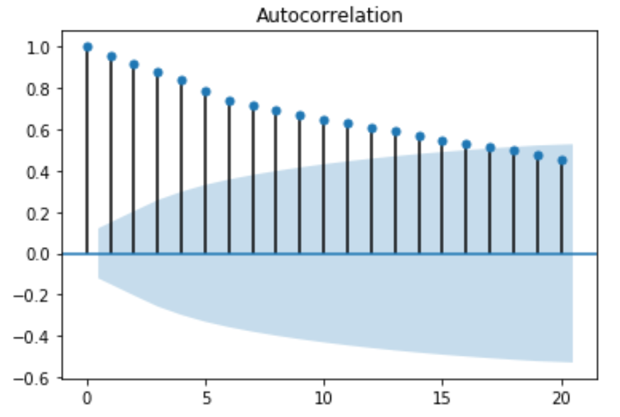
Autocorrelation function (ACF) Test – The Autocorrelation function checks for correlation between two different data points of a Time Series separated by a lag “h”. For example, the ACF will check for correlation between points #1 and #2, #2 and #3 etc. Similarly, for lag 3, the ACF function will check between points #1 and #4, #2 and #5, #3 and #6 etc.
Autocorrelation function test is mainly used for two reasons:
- For detecting non-randomness in the data and
- For identifying the appropriate time series model for the particular dataset.
So an Autocorrelation Function Test, therefore, is important for providing accurate results.
Python code for ACF-
Once you run the python code above, you get a 2D plot of the autocorrelation with first 20 lags:
Partial autocorrelation function (PACF) – In some cases, the effect of autocorrelation at smaller lags will have an influence on the estimate of autocorrelation at longer lags. For example, a strong lag one, can cause an autocorrelation with lag three. The Partial autocorrelation function (PACF) removes the effect of shorter lag autocorrelation from the correlation estimate at longer lags.
Python code for PACF-
Running the code above brings a 2D representation of the data with partial autocorrelation for the first 20 lags:
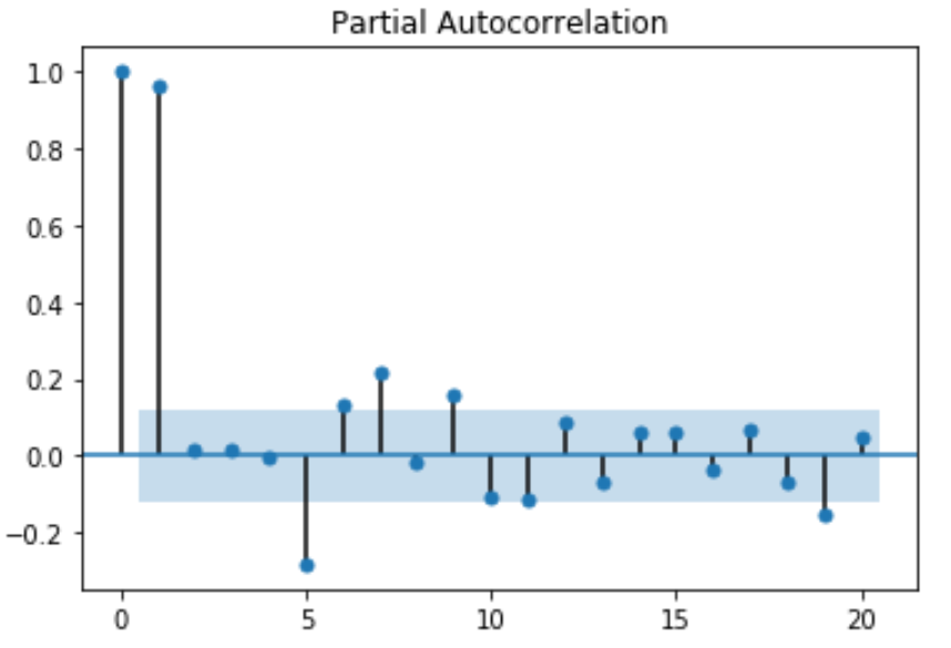
The values of ACF and PACF each vary between plus and minus one. When the values are closer to plus or minus one, it indicates a strong correlation. Moreover, it is a must to note that, if the Time Series is Stationary, the ACF will drop to zero relatively quickly. Whereas, the ACF of Non-Stationary Time Series will decrease slowly. Also, with the ACF graph, we can conclude that the given Time Series is Non-Stationary.
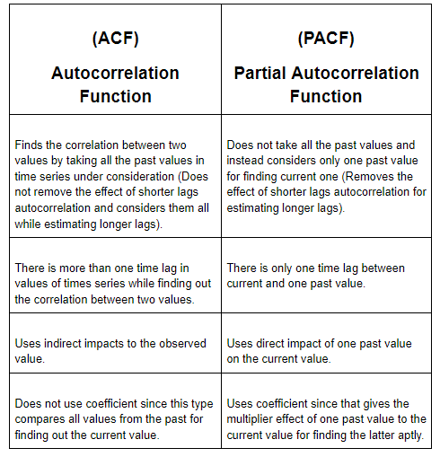
Okay now! Let us explore some differences between ACF and PACF for an easy understanding:
Alright! Let us move further and understand the components of Time Series Analysis which are integral for understanding the different points in a Time Series.
What are the Components of Time Series Analysis?
Basically, a Time Series Analysis takes an entire dataset of a Time Series, which can be divided into three components. These components divide the entire dataset into different categories in accordance with the nature of each value. So, there are three components of a Time Series which are segregated as:
- Trend - The continuance of increasing or decreasing values in a given Time Series.
- Seasonal - The repeating cycle over a specific period (day, week, month, etc.) in a given Time Series.
- Irregular or Random Irregularity (Noise) - The random irregularity of values in a given Time Series.
Another interesting point to note here is that the segregation of the Time Series into all these components is also known as Decomposition. As we have mentioned, a Time Series might include a seasonal component or an irregular component. So, when the segregation of Time Series happens, all kinds of patterns are clearly separated out, which help with the analysis to take place based on each category.
Now, as we know what are the components of Time Series Analysis and why is it important to decompose the Time Series, we must understand 'how' to decompose them as well.
Structures for the Components or Decomposing
As per the nature of the Time Series, it can be presented as an additive or a multiplicative in which each observation is expressed as a sum or a product of the components. On the basis of the seasonal variation, let us learn the two structures for decomposing the Time Series:
- Additive decomposition – If the seasonal variation is relatively constant over time, we can use the additive structure for decomposing a given Time Series. The additive structure is given as -
Xt (Values) = Trend + Random + Seasonal
- Multiplicative decomposition – If the seasonal variation is increasing over time, we can use the multiplicative structure for decomposing a Time Series. The multiplicative structure is given as -
Xt (Values) = Trend * Random * Seasonal
These structures make the separate components of a data be seen as a whole (with either addition or multiplication) based on the seasonal variation’s nature. It is so because the data in trend is dependent on the seasonal data’s movements. This whole data is a better representation of the entire series and helps with accurate predictions.
Moving on, let us find out more on Time Series and see how it helps in forecasting a variable (price, percentage, amount etc.)
What is Time Series Forecasting?
As the name suggests, Time Series forecasting implies predicting those variables that have time as the component. This is an important criterion when it comes to using it for any of the tasks involving machine learning. For example, while using machine learning for predicting stock prices, Time Series Analysis is quite helpful in analysing the factors behind different stock prices in different points in time for forecasting future prices.
Another interesting observation is that the Time Series forecasting can be used in any industry for predicting the future values of a variable. For instance, forecasting the temperature on certain days in the month of December next year based on the current data values.
Now forecasting involves some mathematical and statistical tests taken out from the analysis of past Time Series data for predicting future data. Also, the tests that predict the future dataset accurately, are the ones which are considered the apt ones. Hence, there is a test known as the Granger Causality Test to determine the validity of past data for predicting future values.
Granger Causality Test
The Granger Causality test helps you determine if one Time Series will be useful to forecast another one in the future. It simply mentions that if X leads to Y or X is the contributing factor behind Y, then the prediction based on the past values of both X & Y will outperform the prediction based on only past values of Y.
Also, it is important to note here that this is the oldest concept of causality for Time Series data. For example, It is based on the assumption that:
U - is all the information in the universe
Y - is required to be predicted with all the information in the universe minus information from X so it will be U\X.
X- This Time Series led to Y in the past.
But since we have information about Y’s values in the previous Time Series, we are not including X’s Time Series which determined Y.
The main concept is to discard X and to show that it reduces the predictability of Y since X contained some unique and important information regarding Y. Hence, we say that X-Granger causes Y.
Taking the help of variance, we say that:
σ²(Yᵢ|𝒰ᵢ) < σ²(Yᵢ|𝒰ᵢ\𝒳ᵢ)
In the equation above, X and Y are Stationary stochastic (random) processes.
𝒰ᵢ=(Uᵢ₋₁,…,Uᵢ₋∞) - information in the universe until the time i.
𝒳ᵢ=(Xᵢ₋₁,…,Xᵢ₋∞) - information in the X until the time i.
σ²(Yᵢ|𝒰ᵢ) - the variance of predicting Yi using Ui at the time i.
σ²(Yᵢ|𝒰ᵢ\𝒳ᵢ) - the variance of predicting Yi using all the information in Ui ( time i ) except Xi.
Now, accordingly, if σ²(Yᵢ|𝒰ᵢ) < σ²(Yᵢ|𝒰ᵢ\𝒳ᵢ) then it is clear that X Granger causes Y or X=>Y.
Hence, the Granger Causality test mentions that the prediction of one variable in a Time Series depends on all of its contributing factors in a previous Time Series.
Now let us move to Simple Linear Forecasting Model and find out how this model helps in forecasting a single variable or any number of variables keeping a Time Series as the component.
Simple Linear Forecasting Model
We will discuss a simple linear forecasting model assuming the Time Series is Stationary and doesn’t have seasonality. The basic assumption here is that the Time Series follows a linear trend. The model can be represented as:
Forecast (t) = a + b X t
Here 'a' is the intercept that Time Series makes on Y-axis and 'b' is the slope. Let us now look at the computations of a and b. Consider a Time Series with values D(t) for the time period 't'.
In this equation, 'n' is the sample size. We can validate our model by calculating the forecasted values of D(t) using the above model and comparing the values against actual observed values. We can compute the mean error which is the mean value of the difference between the forecasted D(t) and the actual D(t).
In our stock data, D(t) is the adjusted closing price of MRF. We will now compute the values of a, b, forecasted values and their errors using python.
Note that we are fetching historical data of the "MRF" stock starting 1st Jan 2012 till 31st Dec 2017
The above code gives the output as shown.
The slope of the linear trend (b) is: 41.174491162345355
The intercept (a) is: 1269.3446503776584
We can now check the validity of our model by computing the forecasted values and computing the mean error in python.
The output is as shown:
The mean error is: 8.916373244192283e-12
Does this mean our data is free from seasonality? Do let me know in the comments.
Ahead, let us see how to import, calculate, and plot Time Series Data in Python.
How to Import, Calculate & Plot Time Series Data in Python for forecasting?
Our main focus will be on generating a static forecasting model. We will also check the validity of the forecasting model by computing the mean error. However, before moving on to building the model, we will briefly touch upon some other basic parameters of Time Series like moving average, trends, seasonality, etc.
Importing Data
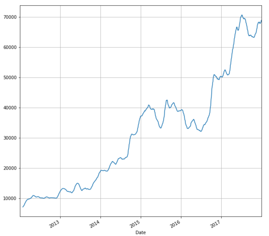
We have imported the necessary libraries at the start of this article and as we have seen above, we will be using the past five years of ‘adjusted price’ of MRF.
We can plot the adjusted price against time using the matplotlib library which we have already imported.
stock['Adj Close'].plot(figsize=(10,10),grid =True)
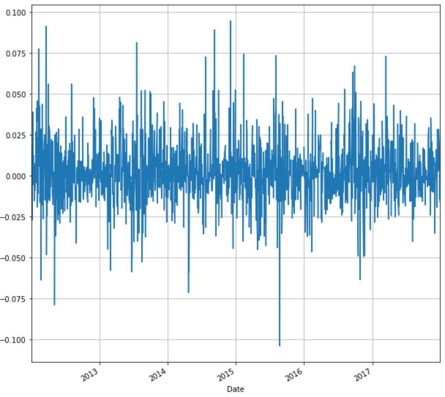
Using Time Series, we can compute daily returns and plot returns against time. We will compute the daily returns from the adjusted closing price of the stock and store in the same dataframe ‘stock’ under the column name ‘ret’. We will also plot the daily returns against time.
stock['ret'] = stock['Adj Close'].pct_change()
stock['ret'].plot(figsize=(10,10),grid=True)
Similar to returns, we can calculate and plot the moving average of the adjusted close price. Moving average is a very important metric used widely in technical analysis. For illustration purpose, we will compute 20 days moving average.
stock['20d'] = stock['Adj Close'].rolling(window=20, center=False).mean()
stock['20d'].plot(figsize=(10,10),grid=True)
Now, let us see how to work with Date-Time Data in Python.
Time Series Analysis: Working With Date-Time Data In Python
Since traders deal with loads of historical data, and need to play around and perform analysis, Date-Time Data is important. These tools are used to prepare the data before doing the required analysis. We will majorly focus on how to deal with dates and frequency of the Time Series. Also, we will discuss indexing, slicing and slicing operations on Time Series. For this blog, we will extensively use the ‘datetime’ library.
Let us begin with importing this library in our program in python:
# Importing the required modules
from datetime import datetime
from datetime import timedelta
Hence, the basic tools are discussed here ahead to make the concept clearer.
To begin with, let us save the current date and time in a variable ‘current_time’. The below code will execute the same.
# Printing the current date and time
current_time = datetime.now()
current_time
datetime.datetime(2020, 2, 22, 1, 18, 57, 478280)
Of course, depending on the time you are running the code, the output will change. We can compute the difference between two dates using datetime.
# Calculating the difference between two dates (14/02/2018 and 01/01/2018 09:15AM)
delta = datetime(2018,2,14)-datetime(2018,1,1,9,15)
delta
Output: datetime.timedelta(43, 53100)
We can convert the output in terms of days or seconds using:
# Converting the output to days
delta.days
Output: 43
If we want to convert it into seconds, we can use the following code.
# Converting the output to seconds
delta.seconds
Output: 53100
If we want to shift a date, we can use the timedelta module which we have already imported.
# Shift a date using timedelta
my_date = datetime(2018,2,10)

# Shift the date by 10 days
my_date + timedelta(10)
Output: datetime.datetime(2018, 2, 20, 0, 0)
We can also use multiples of timedelta function.
# Using multiples of timedelta function
my_date - 2*timedelta(10)
Output: datetime.datetime(2018, 1, 21, 0, 0)
We have seen ‘datetime’ and ‘timedelta’ data types of datetime module. Let us give a brief note of major data types which are of great use while analysing Time Series.
We can convert a datetime format to a string and save it under a string variable, let us see how.
Conversion Between Strings And DateTime
As we mentioned about the conversion of a datetime format, the reverse can also be done and a string which represents a date can be converted to datetime data type.
Output:
'2018-02-14 00:00:00'
datetime.datetime(2018, 2, 14, 0, 0)
We can also use pandas to handle dates. Let us first import pandas.
Output:
DatetimeIndex(['2018-01-14', '2018-02-14'], dtype='datetime64[ns]', freq=None)
In pandas, a missing time or NA values in time are represented as NaT (Not a Time).
Let us now understand ahead indexing and slicing of a Time Series.
Indexing And Slicing Of A Time Series
To understand various operations on a Time Series, let us create a Time Series using random numbers.
Output:
2011-01-02 1.380330
2011-01-05 -0.765646
2011-01-07 0.983679
2011-01-08 0.338122
2011-01-10 -0.919227
2011-01-12 0.577716
The elements of this Time Series can be called like any other pandas series using the index as shown. ts['01/02/2011'] or ts['20110102'] will give the same output 1.380330.
The slicing is also similar to what we have for other pandas series.
# Slicing the Time Series
ts[datetime(2011,1,7):]
Output:
2011-01-07 0.983679
2011-01-08 0.338122
2011-01-10 -0.919227
2011-01-12 0.577716
Now, let us see what happens if your Time Series contains duplicated indices.
Duplicate Indices in Time Series
Sometimes your Time Series may contain duplicated indices. Let us consider the Time Series below.
Output:
2018-01-01 2.081558
2018-01-02 -0.887678
2018-01-02 1.150759
2018-01-02 -1.068980
2018-01-03 0.53671
In the above Time Series, we can see that ‘2018-01-02’ is repeated thrice. We can check this using ‘is_unique’ property of ‘index’ function.
dup_ts.index.is_unique
Output: False
We can aggregate the records with the same index using ‘groupby’ functionality.
grouped=dup_ts.groupby(level=0)
We can now use mean, count or the sum of those records as per our requirement.
grouped.mean()
Output:
2018-01-01 2.081558
2018-01-02 -0.268633
2018-01-03 0.536711
grouped.count()
Output:
2018-01-01 1
2018-01-02 3
2018-01-03 1
grouped.sum()
Output:
2018-01-01 2.081558
2018-01-02 -0.805899
2018-01-03 0.536711
Also, let us see how we can shift the index of the Time Series.
Data Shifting
Here, we will understand how using the ‘shift’ function we can shift the index of the Time Series.
# Shifting the Time Series
ts.shift(2)
Output:
2011-01-02 NaN
2011-01-05 NaN
2011-01-07 -0.079783
2011-01-08 1.286886
2011-01-10 0.961793
2011-01-12 2.532836
There is yet another concept known as Mean Reversion in Time Series Analysis in forecasting the Time Series.
Mean Reversion in Time Series Analysis
Time Series Analysis comprises of techniques for analyzing Time Series data in an attempt to extract useful statistics and identify characteristics of the data. Time Series Forecasting is the use of a mathematical model to predict future values based on previously observed values in the Time Series data.
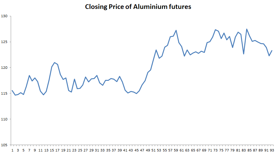
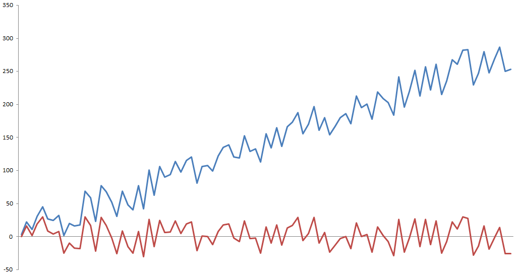
Let us now take a look at the graph below, which represents the daily closing price of Aluminium futures over a period of 93 trading days, which is a Time Series.
Now, what does Mean Reversion Trading imply?
Learning about this very important concept which is Time Series, Mean Reversion is an important inclusion. Well, Mean reversion trading is yet another crucial theory which suggests that prices, returns, or various economic indicators tend to move to the historical average or mean over time. This theory has led to many trading strategies which involve the purchase or sale of a financial instrument whose recent performance has greatly differed from their historical average without any apparent reason.
For example, let the price of gold increase on an average by INR 10 every day and one day the price of gold increases by INR 40 without any significant news or factor behind this rise, then by the mean reversion principle we can expect the price of gold to fall in the coming days such that the average change in price of gold remains the same. In such a case, the mean revisionist would sell gold, speculating the price to fall in the coming days. Thus, making profits by buying the same amount of gold he had sold earlier, now at a lower price.
A mean-reverting Time Series is plotted below to make the understanding easy. Here, the horizontal black line represents the mean and the blue curve is the Time Series which tends to revert back to the mean.
Also, it is important to note here that the collection of random variables is defined to be a stochastic or random process. A stochastic process is said to be Stationary if its mean and variance are constant over time. Furthermore, a Stationary Time Series will be mean reverting in nature, i.e. it will tend to return to its mean and fluctuations around the mean will have roughly equal amplitudes. Also, a Stationary Time Series will not drift too far away from its mean because of its finite constant variance.
Whereas, a Non-Stationary Time Series, on the contrary, will have a time varying variance or a time varying mean or both, and will not tend to revert back to its mean.
In the financial industry, traders take advantage of the Stationary Time Series by placing orders when the price of security deviates considerably from its historical mean, speculating the price to revert back to its mean.
Let us also observe that, in Non-Stationary, data tends to be unpredictable and cannot be modeled or forecasted. A Non-Stationary Time Series can be converted into a Stationary Time Series by either differencing or detrending the data.
Here, a random walk (the movements of an object or changes in a variable that follow no discernible pattern or trend) can be transformed into a Stationary series by differencing (computing the difference between Yt and Yt -1).
Shown below is a plot of a Non-Stationary Time Series with a deterministic trend (Yt = α + βt + εt) represented by the blue curve and its detrended Stationary Time Series (Yt - βt = α + εt) represented by the red curve.
Going ahead, we will now see Trading Strategies based on Mean Reversion.
Trading Strategies based on Mean Reversion
One of the simplest mean reversion trading related trading strategies is to find the average price over a specified period, followed by determining a high-low range around the average value from where the price tends to revert back to the mean. The trading signals will be generated when these ranges are crossed - placing a sell order when the range is crossed on the upper side and a buy order when the range is crossed on the lower side. The trader takes contrarian positions, i.e. goes against the movement of prices (or trend), expecting the price to revert back to the mean.
This strategy looks too good to be true and it is, it faces severe obstacles. The lookback period of the moving average might contain a few abnormal prices which are not characteristic to the dataset, this will cause the moving average to misrepresent the security’s trend or the reversal of a trend. Secondly, it might be evident that the security is overpriced as per the trader’s statistical analysis, yet he cannot be sure that other traders have made the exact same analysis. Because other traders don’t see the security to be overpriced, they would continue buying the security which would push the prices even higher. This strategy would result in losses if such a situation arises.
Pairs Trading is another strategy that relies on the principle of mean reversion trading. Two co-integrated securities are identified, the spread between the price of these securities would be Stationary and hence mean reverting in nature.
An extended version of Pairs Trading is called Statistical Arbitrage, where many co-integrated pairs are identified and split into a buy and sell basket based on the spreads of each pair. The first step in a Pairs Trading or Stat Arb model is to identify a pair of co-integrated securities.
One of the commonly used tests for checking co-integration between a pair of securities is the Augmented Dickey-Fuller Test (ADF Test). It tests the null hypothesis of a unit root being present in a Time Series sample.
A Time Series which has a unit root, i.e. 1 is a root of the series’ characteristic equation, is Non-Stationary. The augmented Dickey-Fuller statistic, also known as t-statistic, is a negative number. The more negative it is, the stronger the rejection of the null hypothesis that there is a unit root at some level of confidence, which would imply that the Time Series is Stationary. The t-statistic is compared with a critical value parameter, if the t-statistic is less than the critical value parameter then the test is positive and the null hypothesis is rejected.
Now let us see the Co-integration check -ADF test.
Co-integration check - ADF Test
Consider the Python code shown below for checking co-integration:
You can see the output below:
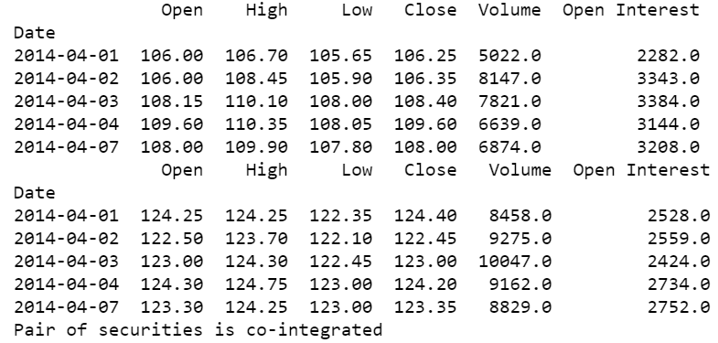
We start by importing relevant libraries, followed by fetching financial data for two securities using the quandl.get() function. Quandl provides financial and economic data directly in Python by importing the Quandl library.
In this example, we have fetched data for Aluminium and Lead futures from MCX. We then print the first five rows of the fetched data using the head() function, in order to view the data being pulled by the code. Using the statsmodels.api library, we compute the Ordinary Least Squares regression on the closing price of the commodity pair and store the result of the regression in the variable named ‘result’.
Next, using the statsmodels.tsa.stattools library, we run the adfuller test by passing the residual of the regression as the input and store the result of this computation the array “ct”.
This array contains values like the t-statistic, p-value, and critical value parameters. Here, we consider a significance level of 0.1 (90% confidence level). “ct[0]” carries the t-statistic, “ct[1]” contains the p-value and “ct[4]” stores a dictionary containing critical value parameters for different confidence levels.
For co-integration we consider two conditions, firstly we check whether the t-stat is lesser than the critical value parameter (ct[0] <= ct[4]['10%']) and secondly whether the p-value is lesser than the significance level (c_t[1] <= 0.1). If both these conditions are true, we print that the “Pair of securities is co-integrated”, else print that the “Pair of securities is not cointegrated”.
To know more about Pairs Trading, Statistical Arbitrage and the ADF test you can check out the self-paced online certification course on “Statistical Arbitrage Trading“ offered jointly by QuantInsti and MCX to learn how to trade Statistical Arbitrage strategies using Python and Excel.
Other Links
So all in all Time Series, its Analysis and Forecasting is quite important and brings us to a great conclusion about it being helpful in predicting Stock prices.
Conclusion
We started with understanding the Time Series as to what it means, why is it important to do the analysis as well as forecasting on the basis of it, and how is it done. Coming down to the conclusion, it is an important concept for predicting variables. The article helped with the core points like:
- Basic functionalities which are of great use in analyzing a Time Series.
- Different types of Time Series and their significance, calculation and plotting with python
- A simple model to forecast Time Series based on trend assuming that the Time Series is free from seasonality.
- Working with Date-Time data and Mean Reversion
Disclaimer: All data and information provided in this article are for informational purposes only. QuantInsti® makes no representations as to accuracy, completeness, currentness, suitability, or validity of any information in this article and will not be liable for any errors, omissions, or delays in this information or any losses, injuries, or damages arising from its display or use. All information is provided on an as-is basis.