RNN, LSTM, and GRU For Trading

By Umesh Palai

This is your complete guide to the steps on installing TensorFlow GPU. We are going to use TensorFlow v2.13.0 in Python to coding this strategy. You can access all python code and dataset from my GitHub a/c.

If you have not gone through my previous article yet, I would recommend going through it before we start this project. In my previous article, we have developed a simple artificial neural network and predicted the stock price. However, in this article, we will use the power of RNN (Recurrent Neural Networks), LSTM (Short Term Memory Networks) & GRU (Gated Recurrent Unit Network) and predict the stock price.

If you are new to Machine Learning and Neural Networks, I would recommend you to go through some basic understanding of Machine Learning, Deep Learning, Artificial Neural network, RNN (Recurrent Neural Networks), LSTM (Short Term Memory Networks) & GRU (Gated Recurrent Unit Network) etc.

Topics covered:

Coding the Strategy

We will start by importing all the libraries. Please note if the below library not installed yet you need to install first in anaconda prompt before importing or else your python will throw an error message

I am assuming you are aware of all the above python libraries that we are using here.

Importing the dataset

In this model, we are going to use daily OHLC data for the stock of “RELIANCE” trading on NSE for the time period from 1st January 1996 to 30 Sep 2018.

We import our dataset.CSV file named ‘RELIANCE.NS.csv’ saved in the personal drive in your computer. This is done using the pandas library, and the data is stored in a dataframe named dataset.

We then drop the missing values in the dataset using the dropna() function. We choose only the OHLC data from this dataset, which would also contain the Date, Adjusted Close and Volume data.

Scaling data

Before we split the data set we have to standardize the dataset. This process makes the mean of all the input features equal to zero and also converts their variance to 1. This ensures that there is no bias while training the model due to the different scales of all input features.

If this is not done the neural network might get confused and give a higher weight to those features which have a higher average value than others. Also, most common activation functions of the network’s neurons such as tanh or sigmoid are defined on the [-1, 1] or [0, 1] interval respectively.

Nowadays, rectified linear unit (ReLU) activations are commonly used activations which are unbounded on the axis of possible activation values. However, we will scale both the inputs and targets.

We will do Scaling using sklearn’s MinMaxScaler.

Splitting the dataset and Building X & Y

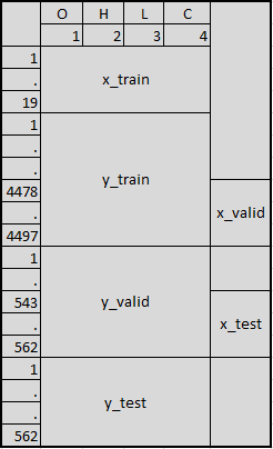
Next, we split the whole dataset into train, valid and test data. Then we can build X & Y. So we will get x_train, y_train, x_valid, y_valid, x_test & y_test. This is a crucial part.

Please remember we are not simply slicing the data set like the previous project. Here we are giving sequence length as 20.

Our total data set is 5640. So the first 19 data points are x_train. The next 4497 data points are y_train out of which last 19 data points are x_valid. The next 562 data points are y_valid out of which last 19 data are x_test.

Finally, the next and last 562 data points are y_test. I tried to draw this just to make you understand.

Building the Model

We will build four different models – Basic RNN Cell, Basic LSTM Cell, LSTM Cell with peephole connections and GRU cell. Please remember you can run one model at a time. I am putting everything into one coding.

Whenever you run one model, make sure you put the other model as a comment or else your results will be wrong and python might throw an error.

Parameters, Placeholders & Variables

We will first fix the Parameters, Placeholders & Variables to building any model. The Artificial Neural Network starts with placeholders.

We need two placeholders in order to fit our model: X contains the network's inputs (features of the stock (OHLC) at time T = t) and Y the network's output (Price of the stock at T+1).

The shape of the placeholders corresponds to None, n_inputs with [None] meaning that the inputs are a 2-dimensional matrix and the outputs are a 1-dimensional vector.

It is crucial to understand which input and output dimensions the neural net needs in order to design it properly. We define the variable batch size as 50 that controls the number of observations per training batch.

We stop the training network when epoch reaches 100 as we have given epoch as 100 in our parameter.

Designing the network architecture

Before we proceed, we have to write the function to run the next batch for any model. Then we will write the layers for each model separately.

Please remember you need to put the other models as a comment whenever you running one particular model. Here we are running only RNN basic so I kept all others as a comment. You can run one model after another.

Cost function

We use the cost function to optimize the model. The cost function is used to generate a measure of deviation between the network’s predictions and the actually observed training targets.

For regression problems, the mean squared error (MSE) function is commonly used. MSE computes the average squared deviation between predictions and targets.

Optimizer

The optimizer takes care of the necessary computations that are used to adapt to the network’s weight and bias variables during training. Those computations invoke the calculation of gradients that indicate the direction in which the weights and biases have to be changed during training in order to minimize the network’s cost function.

The development of stable and speedy optimizers is a major field in neural network and deep learning research. (Learn neural network trading in detail in the Quantra course).

In this model we use Adam (Adaptive Moment Estimation) Optimizer, which is an extension of the stochastic gradient descent, is one of the default optimizers in deep learning development.

Fitting the neural network model & prediction

Now we need to fit the model that we have created to our train datasets. After having defined the placeholders, variables, initializers, cost functions and optimizers of the network, the model needs to be trained. Usually, this is done by mini batch training.

During mini batch training random data samples of n = batch_size are drawn from the training data and fed into the network. The training dataset gets divided into n / batch_size batches that are sequentially fed into the network. At this point the placeholders X and Y come into play. They store the input and target data and present them to the network as inputs and targets.

A sampled data batch of X flows through the network until it reaches the output layer. There, TensorFlow compares the model's predictions against the actual observed targets Y in the current batch.

Afterwards, TensorFlow conducts an optimization step and updates the network parameters, corresponding to the selected learning scheme. After having updated the weights and biases, the next batch is sampled and the process repeats itself. The procedure continues until all batches have been presented to the network.

One full sweep over all batches is called an epoch. The training of the network stops once the maximum number of epochs is reached or another stopping criterion defined by the user applies.

We stop the training network when epoch reaches 100 as we have given epoch as 100 in our parameter.

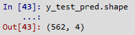
Now we have predicted the stock prices and saved as y_test_pred. We can compare these predicted stock prices with our target stock prices which is y_test.

Just to check no of output, I run the below code and its 562 which is matching with y_test data.

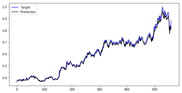
Let's compare our target and prediction. I put both target (y_test) & prediction (y_test_pred) closing price in one data frame named as “comp”.

Now I put both prices in one graph, let see how it looks.

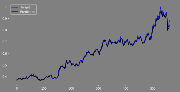
Now we can see, the results are not bad. The prediction values are exactly the same as the target value and moving in the same direction as we expect. You can check the difference between these two and compare the results in various ways & optimize the model before you build your trading strategy.

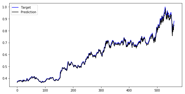
LSTM

Now we can run the Basic LSTM model and see the result.

LSTM with peephole

Let's run the LSTM with peephole connections model and see the result.

GRU

Let's run the GRU model and see the result.

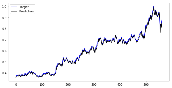
You can check and compare the results in various ways & optimize the model before you build your trading strategy.

Conclusion

The objective of this project is to make you understand how to build a different neural network model like RNN, LSTM & GRU in python tensor flow and predicting stock price.

You can optimize this model in various ways and build your own trading strategy to get a good strategy return considering Hit Ratio, drawdown etc. Another important factor, we have used daily prices in this model so the data points are really less only 5,640 data points.

My advice is to use more than 100,000 data points (use minute or tick data) for training the model when you are building Artificial Neural Network or any other Deep Learning model that will be most effective.

Now you can build your own trading strategy using the power and intelligence of your machines.

List of files in the zip archive:

Deep Learning RNN_LSTM_GRU
RELIANCE.NS

Disclaimer: All data and information provided in this article are for informational purposes only. QuantInsti^® makes no representations as to accuracy, completeness, currentness, suitability, or validity of any information in this article and will not be liable for any errors, omissions, or delays in this information or any losses, injuries, or damages arising from its display or use. All information is provided on an as-is basis.

Advanced Momentum Trading: Machine Learning Strategies Course