Portfolio Optimization Using Monte Carlo Simulation

By Mandeep Kaur

In the previous blog of this series, we saw how to compute the mean and the risk (or standard deviation) of a portfolio containing 'n' number of stocks, each stock 'i' having a weight of 'w_i'.

In this blog, we will see how to do portfolio optimization by changing these weights. By portfolio optimization, we mean getting a portfolio that meets any of the three conditions based on the investor’s requirements.

Conditions of Portfolio Optimization

1. A portfolio which has the minimum risk for the desired level of expected return.
2. A portfolio which gives the maximum expected return at the desired level of risk (risk as measured in terms of standard deviation or variance).
3. A portfolio which has the maximum return to risk ratio (or Sharpe ratio).

Annual Returns and Standard Deviation

To simplify our analysis in this blog, we will deal with daily returns and standard deviation and will consider only 1 month of stock data (Dec 2017). However, in practice, we work with annual returns and standard deviation. The formulae for converting daily returns and standard deviation to an annual basis are as shown (assuming 252 trading days in a year):

Annual Return = Daily Return * 252 Annual Standard Deviation = Daily Standard Deviation * 252

Let us consider a portfolio consisting of four stocks in banking/financial services sector, namely: Bank of America (BAC), Goldman Sachs (GS), JP Morgan Chase & Co (JPM) and Morgan Stanley (MS).

To start with, we’ll assign random weights to all four stocks, keeping the sum of the weights to be 1. We will compute the return and standard deviation of the portfolio as we did in the previous blog and record it. We will then run Monte Carlo Simulations on our portfolio to get the optimal weights for the stocks. We will use python to demonstrate how portfolio optimization can be achieved. Before moving on to the step-by-step process, let us quickly have a look at Monte Carlo Simulation.

Monte Carlo Simulation

This simulation is extensively used in portfolio optimization. In this simulation, we will assign random weights to the stocks. One important point to keep in mind is that the sum of the weights should always sum up to 1. At every particular combination of these weights, we will compute the return and standard deviation of the portfolio and save it. We’ll then change the weights and assign some random values and repeat the above procedure.

The number of iterations depends on the error that the trader is willing to accept. Higher the number of iterations, higher will be the accuracy of the optimization but at the cost of computation and time. For the purpose of this blog, we will restrict ourselves to 10000 such iterations. Out of these 10000 results for returns and corresponding standard deviation, we can then achieve portfolio optimization by identifying a portfolio that satisfies on any of the 3 conditions discussed above.

Portfolio Optimization Process in Python

Let’s start by importing relevant libraries and fetching the data for the stocks for Dec 2017.

#Import relevant libraries
import pandas as pd
import numpy as np
import pandas_datareader.data as web
import matplotlib.pyplot as plt

#Fetch data from yahoo and save under DataFrame named 'data'
stock = ['BAC', 'GS', 'JPM', 'MS']
data = web.DataReader(stock,data_source="yahoo",start='12/01/2017',end='12/31/2017')['Adj Close']

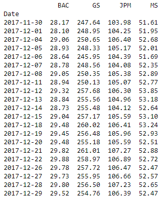
#Arrange the data in ascending order
data=data.iloc[::-1]
print (data.round(2))

The data looks as shown:

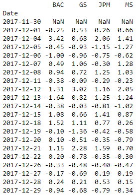
We will then convert these stock prices into returns and will save this under the name ‘stock_ret’.

#Compute stock returns and print the returns in percentage format
stock_ret = data.pct_change()
print (stock_ret.round(4)*100)

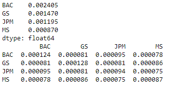
We will now calculate the mean return of all stocks and the covariance matrix.

#Calculate mean returns and covariances of all four the stocks
mean_returns = stock_ret.mean()
cov_matrix = stock_ret.cov()
print (mean_returns)
print (cov_matrix)

Let us define an array to hold the result of each iteration. The array will hold the returns, standard deviation, Sharpe ratio and weights for each step in the iteration. We will define one result array initially containing all zeroes and will save the simulation results in this array. The number of columns in the array is 7 to hold portfolio return, standard deviation, Sharpe Ratio and the weights of all stocks. The number of columns will change with the number of stocks in the portfolio as we have to store the weights for all the stocks. That's why we use the 'len function' while defining the array. The number of rows in the array is equal to the number of iterations.

#Set the number of iterations to 10000 and define an array to hold the simulation results; initially set to all zeros
num_iterations = 10000
simulation_res = np.zeros((4+len(stock)-1,num_iterations))

Let’s now move on to the iterations.

for i in range(num_iterations):
#Select random weights and normalize to set the sum to 1
        weights = np.array(np.random.random(4))
        weights /= np.sum(weights)

#Calculate the return and standard deviation for every step
        portfolio_return = np.sum(mean_returns * weights)
        portfolio_std_dev = np.sqrt(np.dot(weights.T,np.dot(cov_matrix, weights)))

#Store all the results in a defined array
        simulation_res[0,i] = portfolio_return
        simulation_res[1,i] = portfolio_std_dev

#Calculate Sharpe ratio and store it in the array
        simulation_res[2,i] = simulation_res[0,i] / simulation_res[1,i]

#Save the weights in the array
        for j in range(len(weights)):
                simulation_res[j+3,i] = weights[j]

We then save the output in a ‘pandas data frame’ for easy analysis and plotting of data.

sim_frame = pd.DataFrame(simulation_res.T,columns=['ret','stdev','sharpe',stock[0],stock[1],stock[2],stock[3]])
print (sim_frame.head())
print (sim_frame.tail())

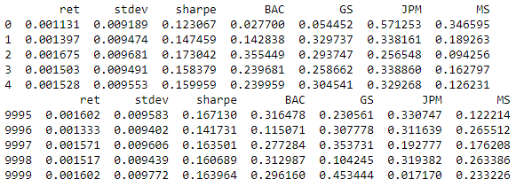
The above output shows some rows of the simulation results. We can now compute the portfolios having maximum Sharpe ratio or minimum risk.

#Spot the position of the portfolio with highest Sharpe Ratio
max_sharpe = sim_frame.iloc[sim_frame['sharpe'].idxmax()]

#Spot the position of the portfolio with minimum Standard Deviation
min_std = sim_frame.iloc[sim_frame['stdev'].idxmin()]
print ("The portfolio for max Sharpe Ratio:\n", max_sharpe)
print ("The portfolio for min risk:\n", min_std)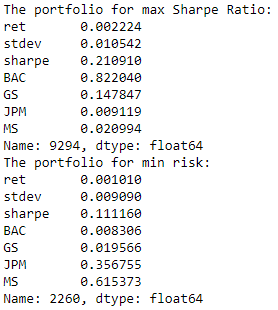

The output can be plotted using the matplotlib library as the relevant points can be highlighted as shown:

#Create a scatter plot coloured by various Sharpe Ratios with standard deviation on the x-axis and returns on the y-axis
plt.scatter(sim_frame.stdev,sim_frame.ret,c=sim_frame.sharpe,cmap='RdYlBu')
plt.xlabel('Standard Deviation')
plt.ylabel('Returns')
plt.ylim(0,.003)
plt.xlim(0.0075,0.012)

#Plot a red star to highlight position of the portfolio with highest Sharpe Ratio
plt.scatter(max_sharpe[1],max_sharpe[0],marker=(5,1,0),color='r',s=600)

#Plot a blue star to highlight position of the portfolio with minimum Variance
plt.scatter(min_std[1],min_std[0],marker=(5,1,0),color='b',s=600)
plt.show()

In the output, the red star shows the portfolio with the maximum Sharpe ratio and the blue star depicts the point with the minimum standard deviation.

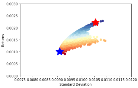
From the above curve, we can get the composition for the required optimal portfolio based on any of the three conditions as discussed above. We can select the portfolio with maximum return for a given risk or a portfolio with minimum risk for a given return or we can simply select the portfolio with maximum Sharpe ratio.

Summary

Just to summarize our complete analysis, we first downloaded the stock price data for one month and computed the mean return of all the stocks and the covariance matrix (which is used in computing the standard deviation of the portfolio). We then ran a Monte Carlo Simulation to compute the risk and return of the portfolio by randomly selecting the weights of the portfolio. We then identify the optimal portfolio based on the Sharpe ratio or other conditions.

Next Step

Our next blog covers various aspects of the portfolio performance evaluation and portfolio performance measurement. It starts with why evaluation and measurement are necessary. Then explains how to compute and analyse the returns generated by the portfolio after a particular time period.

Update

We have noticed that some users are facing challenges while downloading the market data from Yahoo and Google Finance platforms. In case you are looking for an alternative source for market data, you can use Quandl for the same.

Disclaimer: All investments and trading in the stock market involve risk. Any decisions to place trades in the financial markets, including trading in stock or options or other financial instruments is a personal decision that should only be made after thorough research, including a personal risk and financial assessment and the engagement of professional assistance to the extent you believe necessary. The trading strategies or related information mentioned in this article is for informational purposes only.

Download Python Code

• Portfolio Optimization Using Monte Carlo Simulation - Python Code

Login to Download