Updated by Chainika Thakar (Originally written by Devang Singh)
Time series data is simply a collection of observations generated over time. For example, the speed of a race car at each second, daily temperature, weekly sales figures, stock returns per minute, etc.
In the financial markets, a time series tracks the movement of specific data points, such as a security’s price over a specified period of time, with data points recorded at regular intervals. A time series can be generated for any variable that is changing over time.
Further, mean reversion is a simple concept of the stock prices eventually reverting to the mean after deviating from the mean for a certain period of time due to any significant changes in the economy, the organization etc.
Let us find out more about mean reversion in time series with this blog that covers:
- What is time series analysis?
- What is mean reversion?
- Why does mean reversion trading work?
- How does a stock undergo mean reversion in time series?
- Mean reversion in time series with a pair of stocks
- Mean reversion trading strategies with technical indicators
What is time series analysis?
A time series is a sequence of observations indexed over time. In trading, time series forms an important part as it is used to track down the prices of a security over a period of time.
For instance, movement of a security’s price, over a specific period of time recorded at a regular interval.
Pairs Trading: Learn and apply
10 min read
Components of a time series
1. Trend: Trend may show growth or decline in a time series over a long period.
2. Cycles: These are long term oscillations occurring in a time series. These movements generally extend from five to twelve years or more.
3. Seasonality: The periodic fluctuation of time series within a certain period. These fluctuations form a pattern that tends to repeat from one seasonal period to another. Unlike cycles, seasonal behaviour is very strictly regular, meaning there is a precise amount of time between the peaks and troughs of the data.
4. Irregular Fluctuation: These are sudden changes occurring in a time series which are unlikely to repeat. These cannot be explained by trend, seasonal or cyclic movement. This component is sometimes called as random movements in a time series.
Now, time series analysis implies analyzing a time series data to understand its characteristics, design and framework in order to draw inferences from it. Time series analysis has many applications which include yield projections, inventory studies, economic forecasting, sales forecasting etc.
Different methods through which time series analysis can be done include simple forecasting and smoothing models, correlation analysis methods, and ARIMA model.
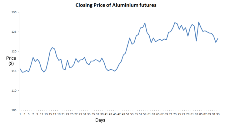
Let us now take a look at the graph below, which represents the daily closing price of Aluminium futures over a period of 93 trading days, which is a Time Series.
Time series analysis is important because it facilitates in:
- Identifying the nature of the phenomenon represented by the sequence of observations in the data.
- Forecasting future values of the time series variable.
- Comparing different time series.
What is mean reversion?
Mean reversion theory suggests that considerable deviations in security prices tend to return to their historical mean.
In other words, if the price moves too far away from its long term average, it will revert to its average. This theory considers only the extreme changes and does not include the normal growth and other market events that take place.
Now that you have an understanding about Mean Reversion, you can learn more about Mean Reversion Trading Strategies to use market data and statistical concepts, here is a brief video.
Use ADF Test to find pairs to trade
10 min read
When the current market price is less than the average price, traders purchase the stock with an expectation that the price will rise. Similarly, When the price is above the average price, investors will sell that security expecting the price to pull back to mean. Pairs trading strategy is based on the mean reversion theory.
For an example, let us assume that the 1 year average price of Stock ABC is $125 and the stock is trading at $150. There may be a gradual increase in the price of the stock over the year due to strong fundamentals but if the stock price increases by 8% within a trading day to $162, then one might short the stock assuming it will return to its long term mean and book a profit.
Why does mean reversion trading work?
Mean reversion trading strategy works since the price is always moving or oscillating around the mean. The reason for the prices reverting to the mean is mainly the sentiments of the traders when the prices deviate from the norm.
Whenever the stock’s price rises in a trend, the traders and investors buy the stocks immediately to avoid missing out on opportunities that a risen price can give. Hence, the demand is more than the supply. This increase in demand also moves the price up further.
As the price continues to rise, more and more traders come into the picture to buy the stock until it reaches a peak where the traders finally start to sell. Now, the role reversal takes place and the supply becomes more than the demand.
In such a situation, the price begins to fall. Forseeing a fall in the price, the majority of the traders start to sell their stocks in fear of losing which leads to surplus in the supply of stocks and the price declines even faster.
Now, at a very low price, some traders begin to buy the stock again pushing the price slightly up. This leads to a balance and hence, the price reverts to the mean.
How does a stock undergo mean reversion in time series?
In the case of mean reversion in time series, the stationarity test plays an integral role.
The stationary test will help you analyse if the time series is stationary or is non-stationary. The time series will be stationary if its mean and variance are constant over time.
Furthermore, a stationary time series will be mean reverting in nature, i.e., it will not drift too far away from its mean because of its finite constant variance.
Whereas, a non-stationary time series, on the contrary, will have a time varying variance or a time varying mean or both, and will not tend to revert back to its mean.
Relevance of stationarity
In the financial industry, traders take advantage of the stationary time series by placing orders when the price of security deviates considerably from its historical mean, speculating the price to revert to its mean.
Shown below is a plot of an asset which is a non-stationary time series with a deterministic trend (Yt = α + βt + εt) represented by the blue curve and its detrended stationary time series (Yt - βt = α + εt) represented by the red curve.
Here, Y-axis represents price of the asset plotted.
Pairs Trading: Learn and apply
10 min read
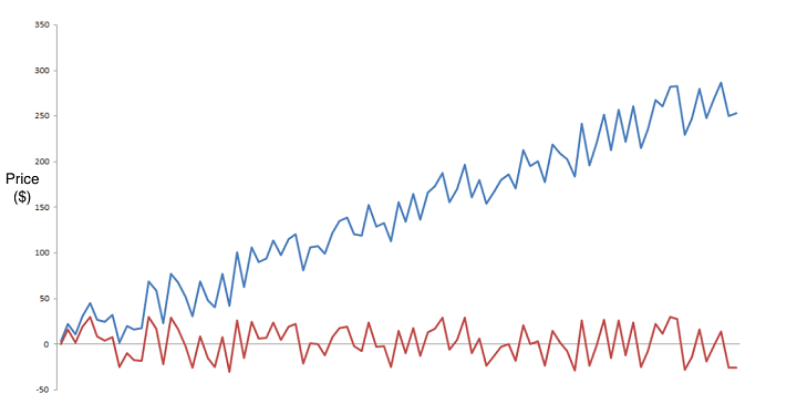
Let us also observe that, in the case of non-stationary time series, data tends to be unpredictable and cannot be modeled or forecasted. A non-stationary time series can be converted into a stationary time series by either differencing or detrending the data.
Here, a random walk (the movements of an object or changes in a variable that follow no discernible pattern or trend) can be transformed into a stationary series by differencing (computing the difference between Yt and Yt -1).
Mean reversion in time series with a pair of stocks
So far we have been observing the stationarity of a single stock over the period of time in the time series analysis. Now, let us find out how to perform the mean reversion with a pair of stocks.
First of all, we check the cointegration between the stocks to find out if they can generate the trading signals together or not. One of the commonly used tests for checking co-integration between a pair of securities is the Augmented Dickey-Fuller Test (ADF Test).
If the result of the ADF test shows that the pair is co-integrated, then the spread between the prices of these securities is stationary. Or else, it is non-stationary.
In the case of stationarity, we will generate the trading signals assuming that the prices of both the stocks will revert to the mean eventually. Hence, we can take the advantage of the prices that deviate from the mean for a short period of time.
If the pair of securities show co-integration, then, we short sell the overvalued stock and for the undervalued stock we go long hoping that the price will rise in future.
Let us see how to perform the cointegration-ADF test on time series with Python.
First of all, you import the necessary libraries and then pull the data for two stocks. Here, we have taken KO (Coca cola) and Pepsi (PEP) as the two stocks.
Now, we will check the cointegration by running the Augmented Dickey Fuller test. Using the statsmodels.api library, we compute the Ordinary Least Squares regression on the closing price of the commodity pair and store the result of the regression in the variable named ‘result’.
Use ADF Test to find pairs to trade
10 min read
Using the statsmodels.tsa.stattools library, we run the adfuller test by passing the residual of the regression as the input and store the result of this computation the array “ct”.
This array contains values like the t-statistic, p-value, and critical value parameters. Here, we consider a significance level of 0.1 (90% confidence level). “ct[0]” carries the t-statistic, “ct[1]” contains the p-value and “ct[4]” stores a dictionary containing critical value parameters for different confidence levels.
For co-integration we consider two conditions:
- Firstly we check whether the t-stat is less than or equal to the critical value parameter (ct[0] <= ct[4]['10%'])
- Secondly, we find out whether the p-value is lesser than the significance level (c_t[1] <= 0.1).
If both these conditions are true, we print that the “Pair of securities is co-integrated”, else print that the “Pair of securities is not co-integrated”.
Let us now check the co-integration between our two stocks i.e., Pepsi and Coca-cola.
Output:
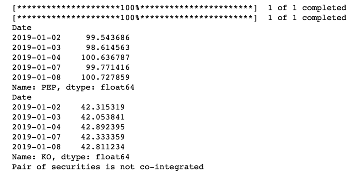
In the above output, you can see that the pair of securities is not co-integrated. Hence, the time series is non-stationary. This means we can not trade with this pair of stocks.
Here's another incredible video by Dr. Ernest Chan. Watch this in-depth video to learn about mean reversion trading strategies.
Mean reversion trading strategies with technical indicators
There are many mean reversion trading strategies but, here we are focussing on the technical indicators for mean reversion strategies. Let us take a look at the mean reversion with three technical indicators namely:
Pairs Trading: Learn and apply
10 min read
Moving Average
A moving average is a technical indicator commonly used with time series data to smoothen the short-term fluctuations and reduce the temporary variation in data. There are three popular types of moving averages for stock market data analysis: Simple Moving Average, Exponential Moving Average, and Weighted Moving Average.
Moving Average also called Rolling average, which is simply the mean or average of the specified data field for a given set of consecutive periods. As new data becomes available, the mean of the data is computed by dropping the oldest value and adding the latest one. So, in essence the mean or average is rolling along with the data, and hence the name ‘Moving Average’.
Also, ‘Moving Average Crossover’ occurs when a short-term simple moving average crosses a long-term simple moving average.
A buy signal is generated when the short-term SMA crosses above the long-term average from below. While a sell signal is triggered when the short-term average crosses below the long-term average from above.
Let us understand the signal generation with the help of the following example:
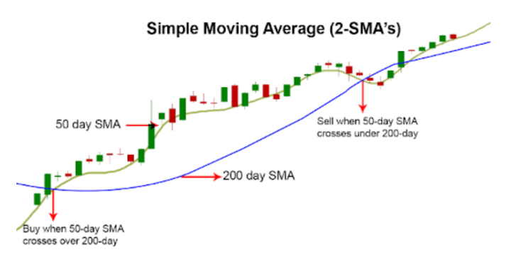
If we look at the long-term 200-day SMA, it is in an uptrend. This is often interpreted as a signal that the market is bullish. When the 50-day SMA crosses above the 200-day SMA, a buy signal is generated, so we will be trading for the uptrend. Conversely, a trader might consider selling when the 50-day SMA crosses below the 200-day SMA.
Hence, in a mean reversion strategy with moving average, we look for a level below the moving average indicating an oversold market. Hence, we will enter the market at a price below the moving average and will exit the market once the price crosses above the moving average.
Now, let us see mean reversion in moving average with the graph below in which Apple Inc is shown in the range bound.

Pairs Trading: Learn and apply
10 min read
In image above, the blue rectangle represents the close price of Apple Inc in the range-bound. The price between the particular period is said to be in the range-bound because every time the price is seen moving away from the mean, it reverts to the mean eventually.
RSI
Relative strength index or RSI Indicator is a momentum oscillator to indicate overbought and oversold conditions in the market. It oscillates between 0 and 100 and its values below a certain value, usually, 30 indicate an oversold market while values above another, say 70, indicate overbought conditions.
Typically, a look back period of 14 days is considered for its calculation and can be changed to fit the characteristics of a particular asset or trading style.
Calculation of RSI involves the following steps:
Average Gain = (previous average gain x 13 + current gain)/14
First average gain = sum of gains in last 14 days/14
Average Loss = (previous average loss x 13 + current loss)/14
First average loss = sum of losses in last 14 days/14
Relative Strength (RS) = Average Gain / Average Loss
RSI = 100 – 100 / (1+RS).
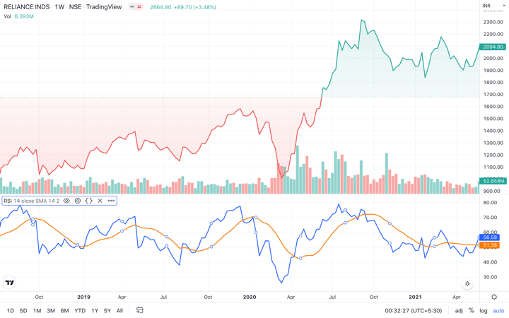
In the chart above, orange line indicates both 14 days RSI plot and the levels for RSI, while the blue line indicates the close price of the stock i.e. Reliance. As discussed above, at below 30, RSI plot is indicating oversold conditions and at above 70, the plot is indicating overbought conditions.
The stock exhibits mean reversion behaviour when the RSI reading is above 70 or below 30. To trade this mean reversion behaviour, we short the asset when RSI is oversold (below 30), expecting the RSI to come back to the mean reading of 51 in order to get favourable returns.
Similarly, we go long when the RSI is overbought (above 70), again for the same reason of making RSI return to the mean of 51.
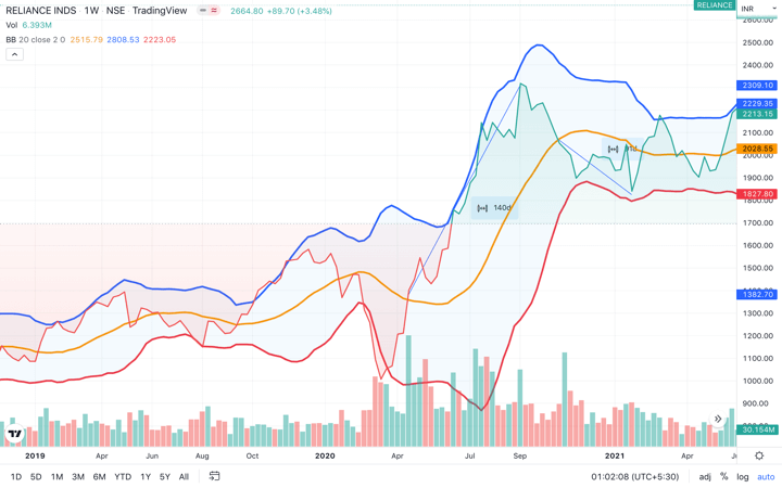
Bollinger Bands
Bollinger Band is a volatility or standard deviation based oscillator which comprises three components. The middle band is a moving average and the other two bands are predetermined, usually two, standard deviations away from the moving average.
As the volatility of the stock prices changes, the gap between the bands also changes. During high volatile market conditions, the gap widens and amid low volatility conditions, the gap contracts.
Bollinger bands involve the following calculations:
- Middle Band or Moving average: 20 Day moving average
- Upper Band: Middle Band + 2 x 20 Day Moving Standard Deviation
- Lower Band: Middle Band – 2 x 20 Day Moving Standard Deviation
Use ADF Test to find pairs to trade
10 min read
As with most technical indicators, values for the look-back period and the number of standard deviations can be modified to fit the characteristics of a particular asset or trading style.
As depicted in the chart above, when the prices continually cross the upper band, the asset is usually in an overbought condition, conversely, when prices are regularly crossing the lower band, the asset is usually in an oversold condition.
Overbought/oversold indicators relies on the concept of mean reversion of the price in the Bollinger Bands. Mean reversion assumes that, if the price deviates substantially from the mean or average, it eventually reverts to the mean price.
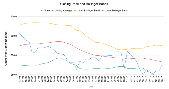
Bollinger Bands find out those asset prices that have deviated from the mean. Let us see in this chart below:
The chart above shows Upper Bollinger Band (blue line), Middle Band (orange line) and Lower Bollinger band (red line).
For Reliance, you can see the range-bound market is visible or 140 days and 91 days represented by two thin light blue lines. In the range-bound markets, mean reversion strategy is known to work the best since the price keeps bouncing between two bands.
It must be noted that the Bollinger Bands do not always give the accurate buy and sell signals. Also, if the trend is strong, there is a risk of the indicator showing overbought or oversold signal too soon, which can lead the trader to place the trade on wrong side.
Now that you understand Mean Reversion in time series, here is a must-watch video, that discusses Mean Reversion and Z-score, mean reversion principles which suggests that prices tend to move around the historical mean over time and z-scores can be used to identify the deviation from the mean and generate the appropriate trading signals.
Conclusion
Mean reversion in time series is the most common strategy used by traders across. Although simple, the mean reversion trading strategy needs to be utilised at the right time in the time series for it to give favourable results. We discussed the basics of mean reversion and also how it works in the time series.
If you also wish to work with mean reversion strategies in time series, you must explore our course on mean reversion trading strategy in Python. This course will help you learn how to create different mean reversion strategies such as Index Arbitrage, Long-Short strategy using market data and advanced statistical concepts.
Note: The original post has been revamped on 13th July 2022 for accuracy, and recentness.
Disclaimer: All investments and trading in the stock market involve risk. Any decision to place trades in the financial markets, including trading in stock or options or other financial instruments is a personal decision that should only be made after thorough research, including a personal risk and financial assessment and the engagement of professional assistance to the extent you believe necessary. The trading strategies or related information mentioned in this article is for informational purposes only.