This article was originally posted on Quants Portal.
In a situation where you wish to determine the returns on investment, one may have all the expertise to do this but without certain information (missing pieces) it would not be possible to derive to a conclusive figure. In practical terms “assume you have the value of all returns of all assets in your portfolio; without the rate at which each asset produces the returns we will not have a true reflection of the portfolio returns at a specific point in time as such we may not provide accurate returns estimate.” A process termed the Hidden Markov model may be used to shed some light in this problem.
The process is split into two components: an observable component and an unobservable or ‘hidden’ component (van Handel, 2008). Nevertheless, from the observable process, we can extract information about the “hidden” processes. As such our task is to determine the unobserved process from the observed one.
The Hidden Markov Models (HMM) has two defining properties. (i) It assumes that the observation at the time was generated by some process whose state is hidden from the observer and (ii) it assumes the state of this hidden process satisfies the Markov property. Complex as it may seem to some, HMM come naturally to understand once one understands what a Markov Model is. We will look up into these two model components then consider advanced techniques that help construct these HMMs.
Constructing A Hidden Markov Model
The “Hidden Process”
A process is said to have the Markov property if:
For any A ⊆ S, any value n and for any time value t1 < t2 < … < tn < tn+1 it is true that
![]()
This means that to determine the next state of the process one can just consider the current the state the process is in and ignore everything that has occurred before as this information is already included in the current state.
We need some properties and definitions that will allow us to help eventually grasp the concept of HMM
- Time Homogeneity: this occurs when the probability of moving from a to b is independent of time, i.e. it does not matter how far you are in the process; as long as the processes are going to move from a to b in one step the probability will be the same throughout. When a process has this property we say this process is Time Homogenous and if not; time non-homogenous
- Though possible to work with infinite states but in our financial context, it suffices to work with a finite amount of states which are irreducible.
- Irreducible States: It is possible to move from any one state to another over a certain number of steps.

This probability matrix is such that:
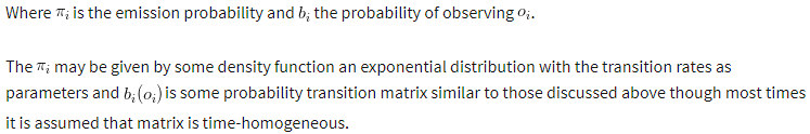
n.b: these emission probabilities are the main drivers of where next the process may go. From our time homogeneity assumption, we can calculate the probability that the process is in state j after t steps given it started at i we multiply the matrix P with itself t times then read off the ijth element of Pn
Example:
Let us consider two probability transition matrices each with two transition states, one that is Time-Homogeneous and one that is not.
The non-Time-Homogeneous case
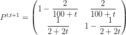
Then ![]() and
and
![]()
Here the probability of changing state depends on where you are in time. Contrary to this procedure, a time-homogenous matrix gives constant probabilities that are independent of time.
![]() On this case
On this case ![]()
Quick task
![]()
![]()
Then ![]()
![]()
Visual representation of Markov transitions
Keeping our analysis simple let us work over a 3 state process S = {1,2,3}
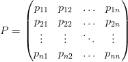
The probability of moving from any one state to any other states is given by the probability matrix P which is given by:
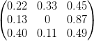
An alternate view of this phenomenon may be given by the following diagram:
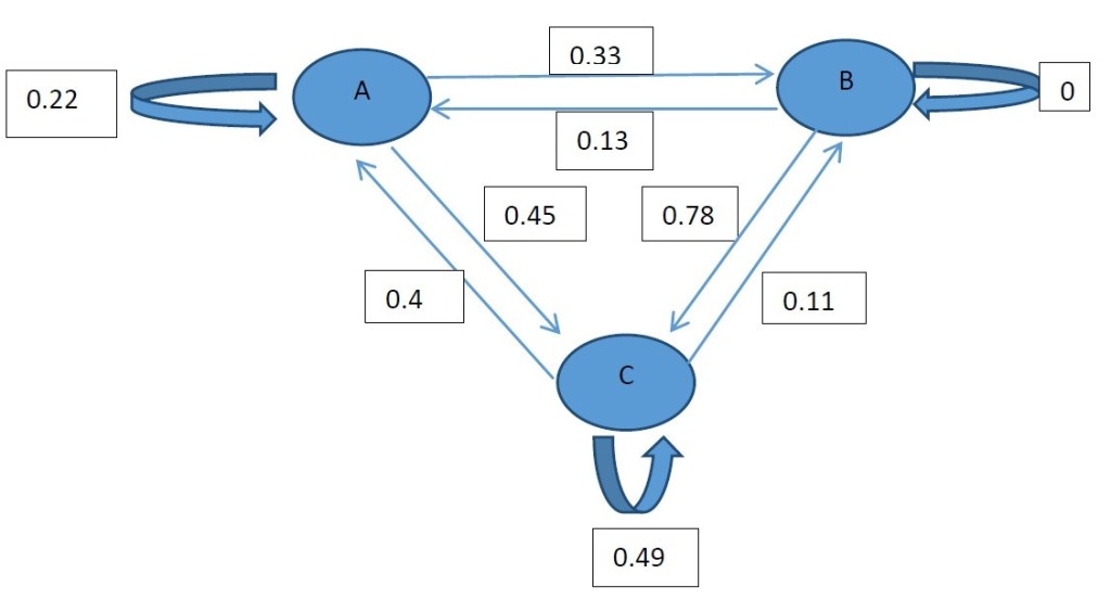
According to the diagram we may move to any state or remain in the current state over one transition (time step). This is true for A and C but once the process is at B it has to move in the next transition, this is because the probability of staying at B is 0.
With the Markov chains, we generate as we shall see that they will hold information on the unobserved and will ultimately yield a more realistic model which is the whole reason we are looking at the HMMs at the first place.
The Observable Process
The hidden states are determined by some properties which we can derive so as to better understand how these hidden states behave.
To derive estimates of the densities of this process we will need to solve numerous systems of equations. Algorithms like the Baum-Welch algorithm and the Viterbi algorithm give extremely accurate estimations but due to their complexity, we will stay clear from them for the time being but return to them later on. Instead, we will look into the Kalman Filter as it follows a procedure similarity to that used in the HMM’s derivation thus it will give us an intuitive understanding of how HMM comes about. Kalman filter is a mathematical technique widely used in control systems and avionics to extract a signal from a series of incomplete and noisy measurements.
Taking a different spin on things I will tabulate the differences between the Kalman filter and the HMM methods first.
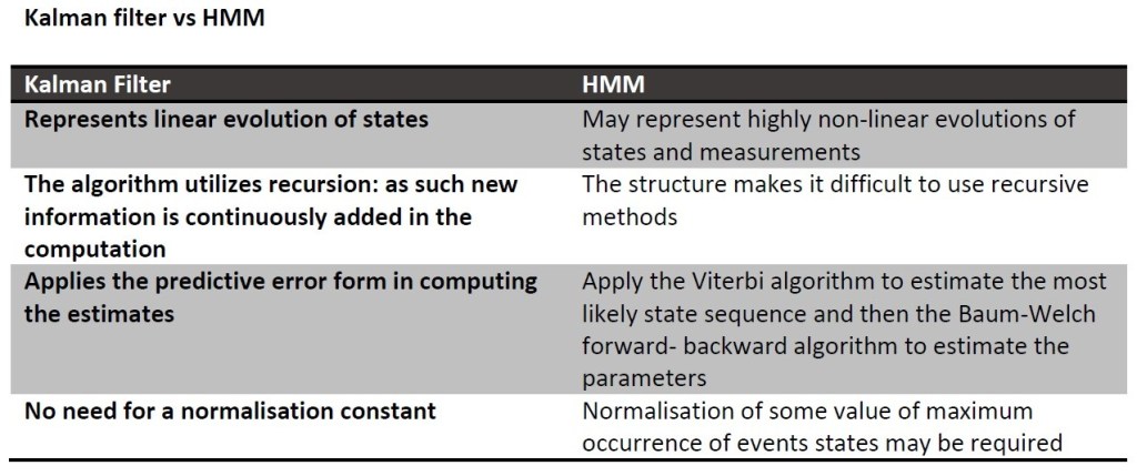
From the above, we get a feeling that finding the estimates is simpler through the Kalman filter but at the same time, we observe how the HMM takes estimation to a whole new level. I drew the table to demonstrate if not allude how imperative it is for one to first be comfortable with the Kalman filter before attempting the finding estimates for the HMM.
Kalman Filter
Key point about the Kalman Filter
- It is a means to find the estimates of the process. Filtering comes from its primitive use of reducing or “filtering out” unwanted variables. Which in our case is the estimation error
Filter Estimates
Suppose we have two processes, a state process and observation process given by the following system of linear equations:
![]()
![]()
Here ${A}{k}$ and ${C}{k}$ can be matrices or variables and can even be as simple as a constant value.
It is common to assume that ${v}{k+1}$ and ${w}{k+1}$ are independently and identically distributed Gaussian or normal distributions with mean 0 and some covariance matrix (ideally diagonal to reflect independence among observations).
The estimates from the Kalman filter equations are derived using fairly advanced methods which require sufficient understanding of multivariate analysis. As such, I will here give the moment equations for the expected value and variance of the hidden process.
The time update equations are
![]()
![]()
And the measurements update equations:
![]()
![]()

The second set of equations (measurements update) determine where the mean and covariance of the process will be given the results of the first set of equations (time update).
The Kalman filter gain (Kk+1) is used to reflect the significance of the error term between our synthesized model versus the some observed (usually historic) model. If the gain which is a probability between 0 and 1 is small it would mean that the estimated model is relatively close reality i.e. a good measure of reality. And if this probability is significantly large, then it may indicate inefficiency in our model and call for re-evaluation with numerous error minimization method available within statistics. The fact is, determining the Kalman gain is just as important as obtaining the estimates of the desired process. The derivation of this filter gain will be provided in an appendix.
Stochastic Dynamic Programming
Eric B. Laber and his colleague Hua Zhou broke down how Dynamic Programming (DP) functions in a simple yet satisfactory and conscious manner. First, they divide the problem (the process) into subintervals. Observing that this “sub-problems” are dependent they propose one to solve the sub-processes individually and store the answer in a table and thereafter using the recorded answers to answer the initial problem.
In any model that contains hidden variables (such as HMMs), the task of determining the sequence of variables is known as decoding (Read, 2011) where the aim is to determine the most likely sequence of the hidden states from the observed sequence (Blunsom, 2004). The Viterbi algorithm has been used to find the single best state sequence for an observed sequence and does so fashion one cannot help but admire.
Viterbi Algorithm
This algorithm follows pretty much a four-step process within which at the end the most likely transition process will be derived.
- Initialization
![]()
- Recursion
![]()
![]()
- Termination
![]()
![]()
Once all transition in the training set the has been accounted for the code will extract the most likely (max probability) event given all the previous events.
- Optimal state sequence backtracking
![]()
The backtracking allows the best state sequence to be found (Blunsom, 2004) from the results from the recursive steps.
Of interest is: given the algorithms ability to obtain the most likely sequence, there is no easy way of obtaining the second best sequence.
Worked example
Bhar and Hamori use HMM to analyse stock market returns among the G7 countries using monthly returns (2004, p. 43). This came about when the pair realized that the USA exerts a strong influence on other G7 countries but find it interesting that the others do not have little or no impact on the US.
Let the model of the entire G7 monthly return be given by a Two-State Markov model of the form
![]()
The returns are split into times when volatilities high and low. The estimated probability of a country remaining in its current state is given by when there is low volatility and if high volatility prevails.
The table below shows the empirical findings from Bhar and Hamori in relation to the seven countries. Given the smoothed probabilities and parameter estimates from the Baum-Welch algorithms and Viterbi algorithms we have:
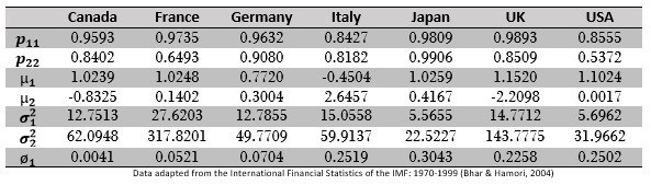
These statistics are not there just to hypothesis models; their main aim is to give more information about the data thus helping decision makers strategize efficiently. Some of the information obtained in this table:
- Japan has the highest propensity to stay in a volatile regime for the longest time and the US is likely to leave volatile periods quicker.
- Italy may obtain more returns on average in a more volatile regime

As an exercise, the reader may take an even closer look to observe what are inferences can be drawn from the data.
Bibliography
Bhar, R., & Hamori, S. (2004). Hidden Markov Models. London: Kluwer Academic Publishers.
Blunsom, P. (2004). Hidden Markov Models.
Read, J. (2011). Hidden Markov Models and Dynamic Programming.
Van Handel, R. (2008). Hidden Markov Models: Lecture notes.
Disclaimer: The views, opinions, and information provided within this guest post are those of the author alone and do not represent those of QuantInsti®. The accuracy, completeness, and validity of any statements made or the links shared within this article are not guaranteed. We accept no liability for any errors, omissions or representations. Any liability with regards to infringement of intellectual property rights remains with them.