
By Nitin Aggarwal and Jasbir Singh
This article is the final project submitted by Jasbir Singh and mentored by Nitin Aggarwal as a part of the coursework in Executive Programme in Algorithmic Trading (EPAT) at QuantInsti. Do check our Projects page and have a look at what our students are building.
Introduction
This article examines profits from trading using the dispersion strategy based on the correlation of stocks, volatility of Index. Dispersion helps the trader take a view on volatility only (assuming that correlation mean reverts) and, therefore, it is made sure that delta risk is hedged by buying or selling futures. In this strategy, both long and short positions are built on volatility and with more strategies available nowadays it is better to use strategies which take advantage of relative values rather than absolutes. This limits the amount of money at risk in one direction.
To be specific, dispersion trading capitalizes on overpricing of index options in relation to individual options when the correlation is high. Depending on the value of correlation between individual stocks, the dispersion can be traded by selling the index options and buying options on index components or by buying index options and selling options on index components.
In recent years there have been many hypotheses as to why dispersion trading is profitable. The most well-received theory is market inefficiency which states that supply and demand in the options market drive the premiums which deviate from their theoretical value. In the study from 1996 to 2005, this was proved when dispersion trading stopped being profitable after 2000.
Strategy
To distinguish dispersion trading, it is simply a hedged strategy which takes advantage of relative value differences in implied volatilities between an index and index component stocks. It involves a short options positions on an index and a long options positions on the components of the index or vice versa. Short positions of straddle or near at the money strangle on the index and long positions of straddles or strangles on 50-60 % of stocks that make up that index are built. The risk posed by the long leg are mitigated by the short positions. Also, the delta exposure is close to zero of at the money straddle and out of the money strangle. Therefore the dispersion strategies are hedged against large market movements and pose a low directional risk.
For index
 where Wi is the weight of the stock ‘i’ in the index. The variance of index can be calculated using the
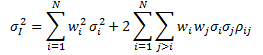 where σI2 is the index variance, wi is the weight for stock in the index. σi2 is the individual stock variance, and ρij is the correlation of stock i with stock j.
The profit in dispersion trading comes from the fact that correlation mean reverts and if one has bought correlation then the realized volatilities of an individual stock will be higher in comparison to the realized volatility of the index. Driessen argues that achieving a profit in dispersion strategy is only possible by the negative correlation risk premium. But it can be achieved from the overpricing of index options in relation to the individual stock options. Hence selling the index option and buying the option on its components and hedging it further with future contracts to remain delta neutral all the time can also be a profitable trade.
The number of options bought or sold doesn't change throughout the trade and the future positions are adjusted according to the delta of the options, by buying or selling of the future contracts.
The profit for a hedged option can be calculated by:
P ≈ θ. (n2-1) + NV-dσ/σ
Where θ = time – decay in dollars; n = standardise move ; N= normalized Vega
Data
The focus of the dispersion trading strategy is Indian Bank Nifty index options and its components bank stocks. We use the 15 minutes data for this strategy.
Implementing the strategy
Steps taken during the projects are as follow:
Implied volatility calculation
To implement this strategy it is important to first calculate the implied volatility of the index Bank Nifty and the stocks in Bank Nifty. Options prices reflect the risk of an instrument either stock or index. The level of risk conveyed by option price is often referred to as implied volatility. The implied volatility of a single-stock option simply reflects the market’s expectation of the future volatility of that stock’s price returns. However, index volatility is driven by a combination of two factors, the individual vol of index components and correlation of index component price returns. By calculating implied volatility, we try to find if the correlation between the stocks is high or low. We use Black-Scholes model to calculate the IV’s. We need time to mature, the strike price, the risk-free interest rate, and the current underlying price. As we are using current month options, from the current price we determine the Option ATM strike and we have the risk-free interest rate.
Implied correlation calculation
We use implied volatility to calculate the implied correlation between stocks. The correlation between the volatility serves as a sign to buy or sell. If implied correlation is high then there is an indication to sell the index options and buy the stock options and vice versa for low implied correlation.
Choosing option
For this strategy, we use a combination of straddle and strangle of both puts and calls. When using this method it is important to hedge the options this can be achieved by investing an equal amount of money into the Bank Nifty index and the stocks of Bank Nifty to achieved a perfectly hedged trade. Time decay: The trades were placed at the start of the month using monthly options and were maintained until expiration. Keeping the trades till expiration helps gain the benefit of time decay on the sold options.
Hedge
This is further hedged using future contracts to keep the whole process delta neutral. Delta of this strategy was adjusted every fifteen minutes when the delta went above 1, one future contract was sold and when the delta dropped to -1 the delta was neutralized by buying one future contract. It is important to keep the delta close to zero for the duration of the trade.
Profit and loss calculation
The PNL for this strategy is coming from two elements one from Options another from future contracts. The future contracts are added to stay delta neutral at the time of expiry all positions are squared off and the final profit is calculated.
Conclusion
Dispersion trading is a very profitable strategy which offers high rewards in response to a low risk, but it is essential to implement the strategy correctly to gain the profit. To make this strategy even better to use it would be easier if the strategy was automated and the hedging was calculated and implemented automatically. With the automated a system it would be easier to implement with an automated system tracking the strategy the hedging calculations can be adjusted in response to the changing in the option prices.
Read our next article that describes developing a fully cloud-based automated trading system that would leverage on mean-reverting or trend-following execution algorithms. This article is the final project submitted by the authors as a part of their coursework in Executive Programme in Algorithmic Trading (EPAT) at QuantInsti.
Disclaimer: The information in this project is true and complete to the best of our Student’s knowledge. All recommendations are made without guarantee on the part of the student or QuantInsti®. The student and QuantInsti® disclaim any liability in connection with the use of this information. All content provided in this project is for informational purposes only and we do not guarantee that by using the guidance you will derive certain profit.