By Chainika Thakar & Varun Divakar
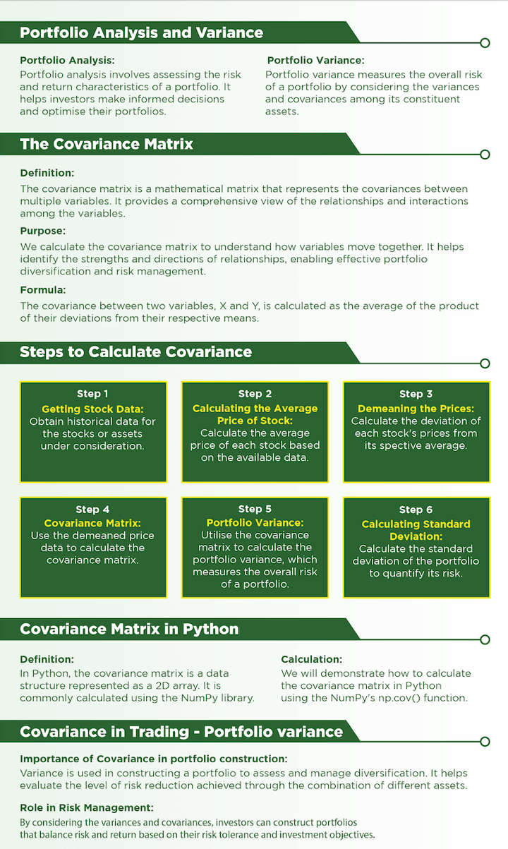
In the world of finance and investment management, effectively managing portfolio risk is essential for achieving optimal returns. Two key concepts that help quantify and analyse risk are the covariance matrix and portfolio variance.
Covariance matrix and portfolio variance are essential tools that provide insights into the relationships between assets and help measure and manage portfolio risk.
The covariance matrix represents the covariances between multiple variables, offering a comprehensive view of their interactions. It plays a critical role in portfolio diversification, risk analysis, and constructing efficient portfolios.
On the other hand, portfolio variance quantifies the overall risk of a portfolio by considering the variances and covariances among its constituent assets.
In brief, the blog covers the following:
All the concepts covered in this blog are taken from the Quantra learning track on Quantitative Portfolio Management. You can take a Free Preview of the course.
In this blog post, we will explore the above mentioned concepts in detail, discussing their calculation and application in portfolio analysis.
This blog covers:
- What is portfolio variance?
- What is the covariance matrix?
- Examples of covariance matrix
- Why do we calculate covariance matrix?
- What is the covariance formula?
- Steps to calculate covariance
- What is a covariance matrix in Python?
- How to calculate covariance in Python for trading?
- Portfolio construction
- Risk assessment
- Formula of portfolio variance
- Example of implementing covariance in portfolio variance
What is portfolio variance?
Portfolio variance is a statistical measure that quantifies the overall risk or volatility of a portfolio of assets. It takes into account the individual variances of the assets in the portfolio as well as the covariances or correlations between them.
Mathematically, the portfolio variance is calculated by considering the weights assigned to each asset in the portfolio, the variances of the individual assets, and the covariances or correlations between pairs of assets.
By assessing the portfolio variance, investors can evaluate the risk level associated with their portfolio and make informed decisions regarding diversification, asset allocation, and risk management strategies. It helps in constructing portfolios that strike a balance between risk and potential returns based on the investor's risk tolerance and investment objectives.
Portfolio variance helps with the process of portfolio analysis. The portfolio analysis is a process of evaluating and managing an investment portfolio to optimise returns while considering the associated risks. It involves assessing the individual assets within the portfolio, their characteristics, and their interactions with each other.
The covariance plays a fundamental role in calculating portfolio variance and is of significant importance in portfolio management.
Hence, we will discuss the covariance matrix first in order to learn more about the portfolio variance.
What is the covariance matrix?
The covariance matrix is a mathematical representation of the covariances between multiple variables.
Covariance is a measure of the joint variability of two random variables.
- If the two variables increase and decrease simultaneously then the covariance value will be positive.
- Conversely if one increases while the other decreases then the covariance will be negative.
The covariance matrix is symmetric, meaning that the covariance between variables X and Y is the same as the covariance between Y and X. Moreover, the diagonal elements of the covariance matrix represent the variances of the individual variables, as the covariance between a variable and itself is its own variance.
The covariance matrix is a fundamental tool in statistics, finance, and data analysis. It is utilised in various applications, including portfolio optimization, risk management, factor analysis, and multivariate analysis. By understanding the covariances between variables, we can gain insights into their interdependencies and make informed decisions based on their relationships.
Examples of covariance matrix
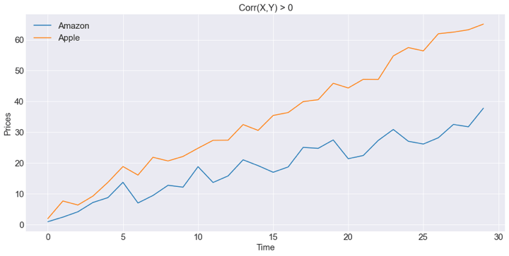
Imagine we have data from four stock prices:
- Amazon
- Apple,
- Walmart, and
- Microsoft
There are two observations in the graphs below.
- At the top, you have a graph in which you could see a positive covariance. When Amazon stock price moves higher, Apple moves in the same positive direction.
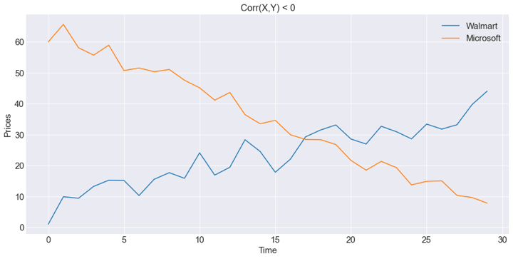
- At the bottom, you can see that, when Microsoft moves down, Walmart does the opposite, moves higher, which means there is a negative Covariance between them.
Why do we calculate covariance matrix?
We calculate the covariance matrix to understand the relationships and interactions between multiple variables. Also, covariance matrix plays an important role in finding out portfolio variance for optimising the portfolio.
Here are the key reasons why we calculate the covariance matrix and how it helps with portfolio:

- Measure of relationship
- Portfolio diversification
- Risk assessment
- Performance evaluation
- Factor analysis
- Multivariate analysis
Measure of Relationship
- Covariance measures the degree to which two variables move together. By calculating the covariances between variables, we can quantify the strength and direction of their linear relationships. This information is valuable in understanding how changes in one variable may affect another and identifying patterns in the data.
Portfolio Diversification
- In finance, the covariance matrix plays a vital role in portfolio management. It helps investors construct diversified portfolios by considering the covariances among different assets. By selecting assets with low or negative covariances, investors can reduce overall portfolio risk and enhance potential returns.
Risk Assessment
- Covariance matrix is essential in evaluating and managing risk. It provides insights into the variability and co-movement of variables. By examining the covariances, we can identify assets or factors that have high correlations and pose potential risks to a portfolio. This information helps in mitigating risk through appropriate diversification or hedging strategies.
Performance evaluation
Variance is used to evaluate the performance of a portfolio over time. By comparing the actual portfolio variance with the expected variance, investors can assess whether the portfolio is performing as expected and whether any adjustments are necessary.
Factor Analysis
- Covariance matrix is used in factor analysis to identify underlying factors driving the variability in a dataset. By examining the covariances among variables, we can determine which variables are influenced by common factors and extract meaningful information from the data.
Multivariate Analysis
- The covariance matrix is a crucial component in multivariate statistical techniques. It is used in various methods such as principal component analysis (PCA), canonical correlation analysis (CCA), and discriminant analysis. These techniques rely on the covariance matrix to identify patterns, reduce dimensionality, and uncover relationships among variables.
Overall, calculating the covariance matrix allows us to quantify relationships, assess risk, construct diversified portfolios, and gain insights from multivariate datasets. It serves as a fundamental tool in various fields, enabling data-driven decision-making and analysis.
What is the covariance formula?
The covariance between two variables, X and Y, can be calculated using the following formula:
$$Cov(X, Y) = \frac{\sum[(X_i - μ_x)(Y_i - μ_y)] }{ (n - 1)}$$Where,
- Cov(X,Y) represents the covariance between variables X and Y.
- Xi and Yi are the individual data points of X and Y, respectively.
- μx and μy represent the means(averages) of X and Y, respectively.
- Σ indicates the sum of the terms.
- n represents the number of data points.
In this formula we calculate the deviation of each data point from the mean for both X and Y, that is,
$$(X_i - μ_x)\;and\;(Y_i - μ_y)$$Then we multiply them together, sum up these products for all data points, and then divide by (n - 1) to obtain the average covariance.
The resulting covariance value indicates the strength and direction of the linear relationship between the two variables. Here is what a positive and negative covariance imply:
- A positive covariance suggests a positive relationship (both variables tend to increase or decrease together),
- A negative covariance indicates an inverse relationship (one variable increases while the other decreases). A covariance of zero implies no linear relationship between the variables.
Steps to calculate covariance
Let us understand in a stepwise manner how to calculate the covariance for two different stocks in the portfolio.
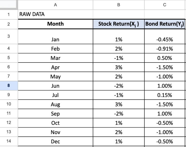
Let us say that there are two stocks in our portfolio that have closed prices as given below.
Step 1 - Getting stock data
Step 2 - Calculating the average price of stock
As you can see each stock consists of the close prices. Using this data, we will first compute the average price for each stock.
In the excel, we will use the formula =AVERAGE(B3:B14) for Stock Return(Xᵢ ) =AVERAGE(C3:14) for Bond Return(Yᵢ).
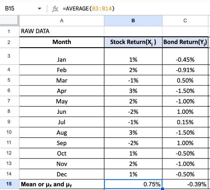
For example, the mean price for Stock Return(Xᵢ ) is given as follows:
$$μ_x = 0.750%$$And the mean price of Bond Return(Yᵢ)is as follows:
$$μ_y = -0.0.39%$$Our ultimate aim is to understand how one stock’s behaviour is related to that of another’s. To compare two stocks with two completely different price ranges, we need to first establish a common base. So to make the comparison of stock movements even, we subtract the mean of the stock price from the stock price.
This will create a new demeaned stock price which will help in comparing how one stock's movement from its mean is dependent on another’s movement from its mean. Let us understand how to create a demeaned series.
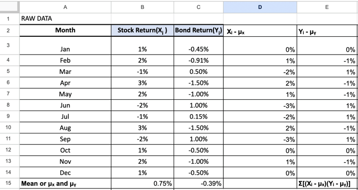
Step 3 - Demeaning the Prices
First, we subtract the mean stock price from the close prices of the corresponding stock. This will give us the matrix with demeaned scores, or a measure of how far a data point is from its mean.
Below you can see that the cell has a formula to subtract B3 from B15 (Average mean value) and each cell till B14 will be subtracted from B15 for each value under Xᵢ - μₓ (Column D).
Similarly, each cell till C14 will be subtracted from C15 (Average mean value) to obtain Yᵢ - μy (Column E).
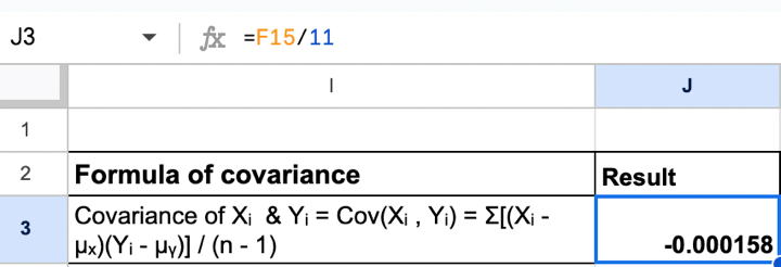
Step 4 - Covariance Matrix
Once we have the demeaned price series, we establish the covariance of different stocks by multiplying the transpose of the demeaned price series with itself and divide it by number of data points, this gives us the covariance matrix.
Below you can see that in one of the cells of the excel sheet, you can do this calculation by giving the formula =F15/11.
This will lead to the following result:
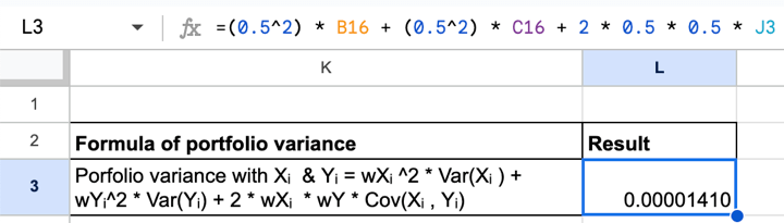
Step 5 - Portfolio Variance
Once we have the covariance of all the stocks in the portfolio, we need to calculate the standard deviation of the portfolio. To do this, we first need to decide the weights or percentage capital allocation for each stock.
While creating the weights matrix we need to keep in mind that the sum of all individual components in the matrix should be equal to 1, since they are a percentage of the total capital invested.
For a portfolio containing two stocks, an equal weight distribution is given by the matrix 'W'.
Below you can see that we have calculated portfolio variance assuming that an equal weight is given to each stock.
Hence, wX = wY = 0.5.
In one of the cells of excel sheet, you can do this calculation in the following manner:
Step 6 - Calculating standard deviation
Once we have calculated the portfolio variance, we can calculate the standard deviation or volatility of the portfolio by taking the square root of the variance.
Variance will be calculated as follows:
- Calculate the variance using the VAR.P or VAR.S function, depending on whether you want to calculate the population or sample variance.
- For population variance, use the formula =VAR.P(B:C)
Columns B and C consist of returns for X and Y (in the portfolio) respectively.
It will look like this in the excel sheet.

The standard deviation was simply calculated with the formula =SQRT(G3).
G3 is the column with Variance of both returns as mentioned above. The square root of variance of both returns gave us the standard deviation of the portfolio.
One can construct various portfolios by changing the capital allocation weights of the stocks in the portfolio.
What is a covariance matrix in Python?
In Python, a covariance matrix is a two-dimensional array or matrix that represents the covariances between multiple variables. It is typically represented using a NumPy array or a pandas DataFrame.
The covariance matrix in Python provides a concise and organised way to store and access the covariances between variables. It is a square matrix where the rows and columns correspond to the variables in the dataset.
For example, let's consider a dataset with three variables: X, Y, and Z. We can calculate the covariance matrix using the “cov” function from NumPy or pandas.
Using NumPy:
Output:
[[10. 10. 5. ]
[10. 10. 5. ]
[ 5. 5. 2.5]]
Using Pandas:
Output:
[[10. 10. 5. ]
[10. 10. 5. ]
[ 5. 5. 2.5]]
Hence, both approaches have generated the same covariance matrix.
The covariance matrix in Python provides a convenient way to access and analyse the covariances between variables in various statistical and financial applications.
How to use covariance in Python for trading?
Covariance can be useful in trading for several purposes, including portfolio construction, risk assessment, and diversification analysis.
Let us discuss the following two examples in which you can utilise covariance in Python for trading.
- Portfolio construction
- Risk assessment
Portfolio Construction
Covariance is crucial in portfolio construction to understand the relationship between different assets and achieve diversification. You can use the covariance matrix to determine the pairwise covariances between the returns of various assets.
To obtain a matrix of asset returns, you typically need historical price data for the assets.
Here's an example of how you can calculate the matrix of asset returns in Python:
Output:

Matrix of Asset Returns:
[[-0.00017424 -0.01023311]
[ 0.00464507 -0.00828998]
[ 0.011385 0.00622974] ...
[-0.03068518 0.03308892]
[ 0.02832432 0.08082691]
[ 0.00246887 0.01116402]]

Covariance Matrix:
[[0.00044494 0.00040597]
[0.00040597 0.00170461]]

Covariance between asset AAPL and asset TSLA: 0.0004059699915867854
The output provides the matrix of asset returns, the covariance matrix, and the covariance between asset AAPL and asset TSLA.
In this case, the covariance between AAPL and TSLA is 0.00040597, indicating a positive relationship between the two assets' returns.
A positive covariance indicates that the returns tend to move in the same direction and not in the opposite directions.
Hence, you can look for opportunities to profit from simultaneous movements in both stocks.
Risk assessment
Covariance is also useful in evaluating and managing risk. It helps quantify the co-movement between assets, which is crucial for understanding portfolio risk. You can calculate portfolio variance using covariance to assess the overall risk of a portfolio.
Here is the python code for risk assessment using covariance of the returns above.
Output:
Portfolio Risk: 0.02720978684223748
A portfolio risk of 0.0272 is considered relatively low.
Lower portfolio risk indicates lower potential volatility or fluctuations in the portfolio's returns.
In the context of risk assessment, a lower portfolio risk is generally desirable for investors who prioritise stability and seek to minimise the potential for large swings in portfolio value. It suggests a more conservative or less volatile investment approach.
Formula of portfolio variance
The formula for portfolio variance depends on the weighting scheme used. Here are the formulas for two common weighting schemes:
Weighting scheme 1
Equal Weighting: In this approach, each asset in the portfolio is assigned an equal weight. Let's assume we have N assets in the portfolio.
Portfolio Variance = (1/N2) * ΣΣ(Covariance_XY)
Where,
- Covariance_XY represents the covariance between asset X and asset Y.
- ΣΣ denotes the sum of the covariances for all pairs of assets.
General Weighting: In this approach, each asset in the portfolio is assigned a specific weight. Let's assume we have N assets in the portfolio, and the weights are represented by w1, w2, ..., wN.
Weighting scheme 2
Portfolio Variance = ΣΣ(wx * wy * Covariance_XY)
Where,
- wx represents the weight of asset X.
- wy represents the weight of asset Y.
- Covariance_XY represents the covariance between asset X and asset Y.
- ΣΣ denotes the sum of the weighted covariances for all pairs of assets.
Example of implementing covariance in portfolio variance
Assume we have two stocks, TSLA and AAPL, and we have historical returns data for a specific period.
TSLA returns: [21.3686676 , 21.14999962, 20.9746666]
AAPL returns: [40.83158112, 40.82447433, 41.01411057]
To calculate the portfolio covariance, we can allocate 60% weightage to TSLA and 40% weightage to AAPL as taken in the Python code earlier.
Step 1:
- For TSLA:
Weighted TSLA Returns = TSLA Returns * Weight Allocation for TSLA
Weighted TSLA Returns = [21.3686676, 21.14999962, 20.9746666] * 0.60
Weighted TSLA Returns = [12.82120056, 12.68999977, 12.58479996] - For AAPL:
Weighted AAPL Returns = AAPL Returns * Weight Allocation for AAPL
Weighted AAPL Returns = [40.83158112, 40.82447433, 41.01411057] * 0.40
Weighted AAPL Returns = [16.33263245, 16.32978973, 16.40564423]
Below you can see the same in Python code.
Output:

Weighted TSLA Returns: [12.82120056 12.68999977 12.58479996]

Weighted AAPL Returns: [16.33263245 16.32978973 16.40564423]
Step 2:
Calculate the covariance between the weighted returns of the two stocks. Covariance between TSLA and AAPL: Cov(Weighted Returns TSLA, Weighted Returns AAPL).
Using the formula for covariance:
$$Covariance = Σ((x_i - μ_x)(y_i - μ_y)) / (n - 1)$$Where,
- xi and yi are the weighted returns for TSLA and AAPL, respectively, at a given time period.
- μx and μy are the means(averages) of the weighted returns for TSLA and AAPL, respectively.
- n is the number of observations (in this case, 4).
The calculation will be as follows:
Covariance = [(0.03 - 0.015)(0.012 - 0.012) + (0.012 - 0.015)(0.016 - 0.012) + (0.018 - 0.015)(0.004 - 0.012) + (0.006 - 0.015)(0.008 - 0.012)] / (4 - 1) = (-0.000003 + 0.000003 + -0.000006 + -0.000006) / 3 = -0.000004
Hence, by summing up the weighted covariance terms, you obtain the portfolio variance.
Output:

Covariance between the weighted returns of TSLA and AAPL: -0.004144490079494139
Hence, the portfolio variance between TSLA and AAPL is -0.000004.
A negative portfolio variance suggests an inverse relationship, where the returns of TSLA tend to move in the opposite direction of the returns of AAPL.
But the negative portfolio variance also depends on your individual risk tolerance. If it fits the risk tolerance then you can continue with this portfolio and keep monitoring to ensure that it does not go beyond your risk tolerance.
Even if the portfolio variance turns out to be positive, you must keep monitoring, rebalancing and optimising your portfolio since the market conditions can keep changing the returns.
Next steps
Since the portfolio covariance is negative, you can:
- Continuously monitor the relationship between the chosen assets’ returns and their covariance. Market dynamics and correlations can change over time, so regularly review and rebalance your portfolio as needed.
- Consider optimising your portfolio by incorporating assets with different risk-return characteristics and covariance patterns. Utilise portfolio optimization techniques to find an optimal allocation that balances risk and return based on your preferences and investment goals.
- Consider combining assets with different covariance patterns to achieve diversification.
Bibliography
- How to Create a Covariance Matrix using Python
- Modern Finance Systems: Theory and applications
- Covariance matrix
- Investment Portfolio: Variance, Weight, and Return
Conclusion
Covariance matrix and portfolio variance are important tools for portfolio analysis and risk assessment in finance. The covariance matrix helps understand relationships between variables, while portfolio variance quantifies overall risk.
These concepts are essential for portfolio diversification, risk management, and informed decision-making in investment management. Python libraries like NumPy and pandas facilitate the calculation and analysis of these metrics and we discussed how to trade with covariance matrix and portfolio variance using Python code.
If you wish to learn more about covariance matrix and portfolio variance, you can explore the course on Quantitative Portfolio Management. This course is recommended for portfolio managers and quants who wish to construct their portfolio quantitatively, generate returns and manage risks effectively.
In this course, you will learn different portfolio management techniques such as Factor Investing, Risk Parity and Kelly Portfolio, and Modern Portfolio Theory.
Download excel file for calculating covariance matrix:
Disclaimer: All data and information provided in this article are for informational purposes only. QuantInsti® makes no representations as to accuracy, completeness, currentness, suitability, or validity of any information in this article and will not be liable for any errors, omissions, or delays in this information or any losses, injuries, or damages arising from its display or use. All information is provided on an as-is basis.